Reconstructing higher-resolution four-dimensional time-varying volumetric data

Figures & data

Figure 1. The illustration of concept of time-varying volumetric data by using the Tornado dataset, which is visualised at four time steps $1,10,20$, and 30. The black axis denotes the time step.

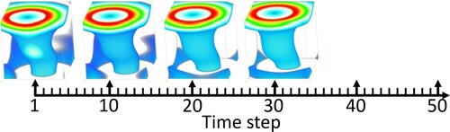
Figure 2. The research framework.

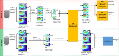
Figure 3. The SSR-DoubleUNetGAN's generator architecture. (a) The schematic diagram of operations. (b) The generator architecture. (c) The Transform Block (TB). (d) The Transform Block & Self-Attention Block (TB&SAB). (e)The Self-Attention Block (SAB).

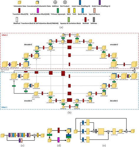
Figure 4. The architecture of the spatial and temporal discriminators.

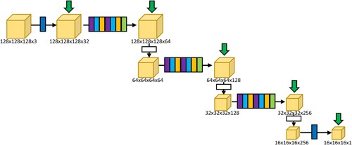
Table 1. The name, dimensions, scaling factor, number of epochs for training, consumed training time and inference time of each dataset.

Dataset	Dimensions($x\times y\times z\times t$)	Scaling factor	Number of epochs	Training time (s)	Inference time (s)
SquareCylinder	192 × 64 × 48 × 102	4	20	651.18	3.19
Hurricane (wind)	250 × 250 × 50 × 48	5	50	1065.46	4.63
Hurricane (QSNOW)	250 × 250 × 50 × 48	5	15	314.97	–
Hurricane (QICE)	250 × 250 × 50 × 48	5	–	–	4.35
ViscousFingers	100 × 100 × 100 × 121	5	12	497.02	4.75
Ionisation (H)	150 × 100 × 100 × 100	5	40	1259.76	4.91

Figure 5. The visualisation of the synthesised high-resolution SquareCylinder dataset from (a) the Ground Truth, (b) our method, (c) SSR-TVD, (d) Tricubic, (e) SRResNet, (f) Cubic, and (g) Linear.

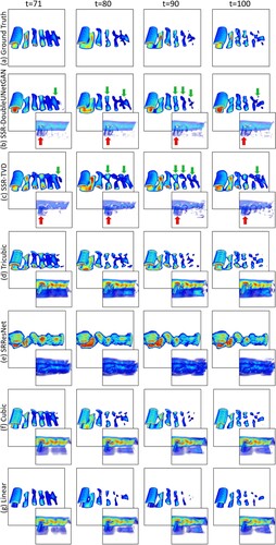
Figure 6. The visualisation of the synthesised high-resolution ViscousFingers dataset from (a) the Ground Truth, (b) our method, (c) SSR-TVD, (d) Tricubic, (e) SRResNet, (f) Cubic, and (g) Linear.

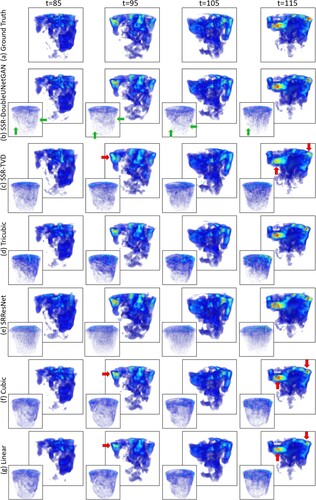
Figure 7. The visualisation of the synthesised high-resolution Hurricane (wind) dataset from (a) the Ground Truth, (b) our method, (c) SSR-TVD, (d) Tricubic, (e) SRResNet, (f) Cubic, and (g) Linear.

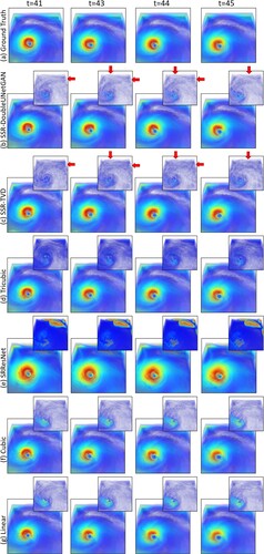
Figure 8. The visualisation of the synthesised high-resolution Hurricane (QICE) from (a) the Ground Truth, (b) our method. In this case, we use the Hurricane (QSNOW) variable to train our model and use the Hurricane (QICE) variable for inference.

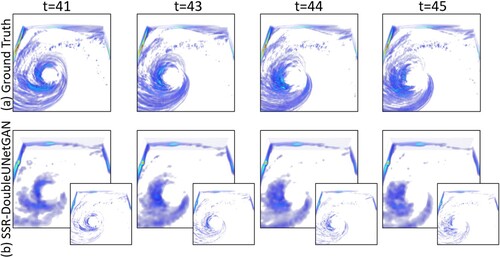
Figure 9. The PSNR and SSIM comparison of different methods in reference to the Ground Truth volumes for (a) SquareCylinder, (b) ViscousFingers and (c) Hurricane (wind) datasets.

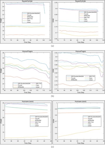
Table 2. The MOS comparison of all methods for each dataset.

Dataset	Our method	SSR-TVD	Tricubic	SRResNet	Cubic	Linear
SquareCylinder	7.8	6.9	7.5	4.2	7.0	7.4
Hurricane (wind)	8.8	8.0	6.8	5.6	7.1	7.5
ViscousFingers	8.3	7.4	8.0	7.1	8.0	7.5

Note: The best scores are indicated in bold.

Table 3. The Frames Per Second (FPS) of our visualisation for each dataset.

Dataset	FPS
SquareCylinder	24
Hurricane (wind)	16
ViscousFingers	9

Table 4. The ablation study of our model.

Model Name	TB	TB&SAB (in encoders/decoders)	TB&SAB (as bridges)	ResPath	Addition
Our method	✓	✓	✓	✓	✓
Model_TBwithoutRes	TB without Residual	TB without Residual&SAB	TB without Residual&SAB	TB without Residual-based ResPath	✓
Model_Conv4TB	Conv	Conv&SAB	Conv&SAB	Conv-based ResPath	✓
Model_NoSAB	✓	TB	TB	✓	✓
Model_ResBlocks4Bridges	✓	✓	Residual Blocks	✓	✓
Model_SkipCon4ResPath	✓	✓	✓	Skip Connection	✓
Model_Multiple4Add	✓	✓	✓	✓	Multiply4Add

Note: For each variant model, only one module is changed.

Figure 10. The PSNR and SSIM values for different models involved in the ablation study of our model.

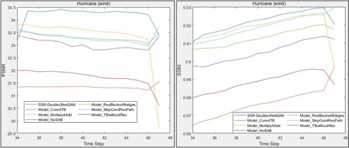
Figure 11. The visualisation of the synthesised high-resolution Ionisation (H) from (a) the Ground Truth, (b) our method, (c) SSR-TVD, (d) Tricubic, (e) SRResNet, (f) Cubic, and (g) Linear.

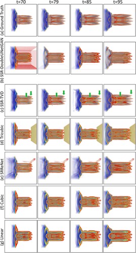
Figure 12. The PSNR and SSIM comparison of all methods inference to the Ground Truth for the Ionisation (H) dataset.

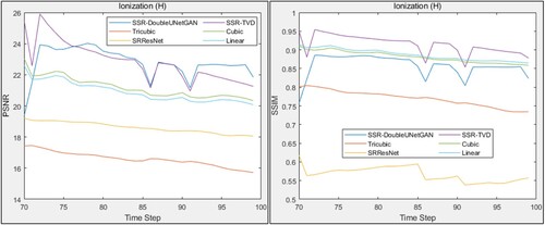
Figure 13. The PSNR values of the synthesised super-resolution volumes from our model at multiple number of epochs for the SquareCylinder dataset.

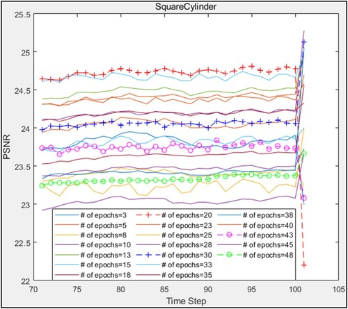
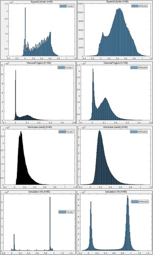
Figure 14. The data distribution of the synthesised super-resolution volumes at a random time step (as listed in each figure's title) from the Tricubic (left) and SRResNet (right) techniques for all datasets.

Data availability statement

The data that support the findings of this study are openly available in IEEE SciVis Contest repository at https://sciviscontest.ieeevis.org/.