Development of ic-ELISA and lateral-flow immunochromatographic assay strip for the simultaneous detection of avermectin and ivermectin

Figures & data

Figure 1. The structure of AVM structural analogues: (A) AVM; (B) IVM; (C) DOR; (D) EP and (E) EMM.

Figure 2. The UV–Vis spectra of different antigens. (A) UV–Vis spectra of AVM–BSA immunogens and (B) UV–Vis spectra of AVM–OVA coating antigens.

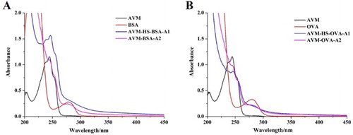
Figure 3. The characterization of obtained mAb 1H2. (A) The antibody subtype analysis of mAb 1H2 and (B) The affinity constant analysis of mAb 1H2.

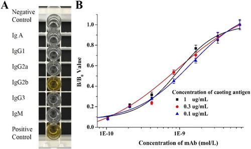
Table 1. The evaluation of different immunogens and coating antigens.

Antigens	AVM–HS–OVA-A1		AVM–OVA–A2
	Titer	IC50 (ng/mL)	Titer	IC50 (ng/mL)
AVM–HS–BSA-A1	81,000	45	27000	5
AVM–BSA-A2	9000	25	9000	−

Figure 4. The optimization of the ic-ELISA method. (A) The optimization of the ic-ELISA method with different pH values; (B) the optimization of the ic-ELISA method with different ionic strengths (NaCl content); (C) the optimization of the ic-ELISA method with different acetonitrile contents and (D) the standard curve established under the optimum condition (AVM and IVM).

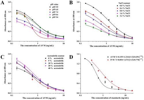
Table 2. The optimization of the ic-ELISA method.

Optimized conditions		Bmax value	IC50 (ng/mL)	Bmax/IC50
pH value	pH 5.0	1.732	0.822	2.11
	pH 6.0	1.527	0.571	2.67
	pH 7.4	1.229	0.893	1.38
	pH 8.6	1.17	0.661	1.77
	pH 9.6	1.588	0.913	1.74
NaCl content (m/v)	0% NaCl	2.10	1.22	1.72
	0.4% NaCl	1.73	0.916	1.89
	0.8% NaCl	1.66	0.614	2.70
	1.6% NaCl	1.21	0.542	2.23
	3.2% NaCl	1.04	0.496	2.10
Acetonitrile content (v/v)	0% Acetonitrile	1.50	0.891	1.68
	5% Acetonitrile	1.69	0.532	3.18
	10% Acetonitrile	1.87	0.621	3.01
	20% Acetonitrile	1.96	0.643	3.05

Table 3. The CR value of mAb 1H2 by the ic-ELISA method.

Analytes	IC50 (ng/mL)	CR (%)
AVM	0.491	100
IVM	0.770	63.8
DOR	>  1000	<  0.1
EP	>  1000	<  0.1
EMM	>  1000	<  0.1

Figure 5. The sensitive analysis of the lateral-flow ICA strip. (A) The sensitive analysis with AVM: (1) 0 ng/ml; (2) 2.5 ng/ml; (3) 5 ng/ml; (4) 10 ng/ml; (5) 25 ng/ml; (6) 50 ng/ml; (B) The sensitive analysis with IVM: (1) 0 ng/ml; (2) 5 ng/ml; (3) 10 ng/ml; (4) 25 ng/ml; (5) 50 ng/ml; (6) 100 ng/ml; (C) the standard curve for AVM with ICA assay; and (D) the standard curve for IVM with ICA assay.

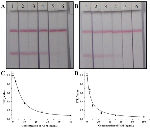
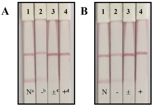
Figure 6. The spiked sample analysis with lateral-flow ICA strip by visual (n = 6).(A) The spiked sample with AVM: (1) 0 ng/ml; (2) 5 ng/ml; (3) 15 ng/ml; (4) 45 ng/ml; (B) The spiked sample with IVM: (1) 0 ng/ml; (2) 15 ng/ml; (3) 45 ng/ml; (4) 135 ng/ml. ^a Negative samples. ^b Negative result. The test line is obviously observed. ^c Weakly positive result. Light test line is observed. ^d Positive result. No test line is observed.

Table 4. The spiked sample analysis with ic-ELISA and lateral-flow ICA strip (n = 6).

Spiked standard	Spiked (ng/g)	Result (ng/g)	Recovery (%)	Spiked standard	Spiked (ng/g)	Result (visual)	Result (ng/g)	Recovery (%)
	2.5	2.72 ± 0.08^a	109		5	−^b	6.24 ± 0.18	125
AVM	5	5.28 ± 0.13	106	AVM	15	±^c	17.52 ± 0.52	117
	10	10.89 ± 0.31	109		45	+^d	– ^e	–
	5	5.58 ± 0.25	112		15	−	16.48 ± 0.67	110
IVM	10	9.78 ± 0.49	98	IVM	45	±	53.64 ± 2.03	119
	20	18.83 ± 0.48	94		135	+	–	–

^aMean value ± standard deviation (n = 6).

^bNegative result. The test line is obviously observed.

^cWeakly positive result. Light test line is observed.

^dPositive result. No test line is observed.

^eWithout result.