Figures & data
Figure 1. Structure and schematic diagram of the ILFST. (a) Positive; (b) Negative
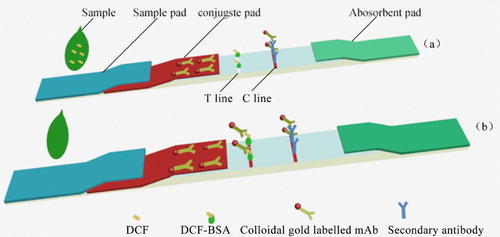
Figure 2. (a) Synthesis of DCF-BSA using activated ester method. (b) Synthesis of DCF-BSA using mixed anhydride method.
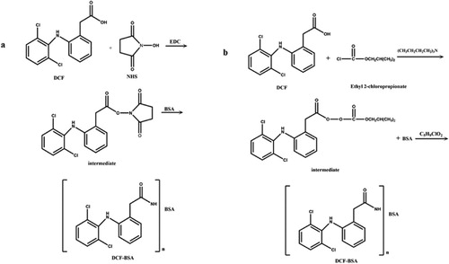
Table 1. Characterization of the optimal antiserum produced by MA and AE methods toward free DCF and coating antigens.
Table 2. Characterization of anti-DCF mAbs by ELISA.
Figure 3. ROD curves from detections of different spiked health wine samples. Blank health wine samples were spiked with DCF to final concentrations of 0, 0.25, 0.50, 1.0, 2.0, 4.0 and 8.0 ng/ml and tested using the ILFST. Relative optical density (ROD) of the test line was read by a TSR3000 membrane strip reader (Bio-Dot).
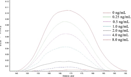
Figure 4. The quantitative calibration curve drawn from testing different DCF standard solutions using ILFST. The X-axis represents the concentrations of DCF in spiked samples. B/B0 represents the percentage of ROD values obtained from spiked samples divided by that of the blank sample.
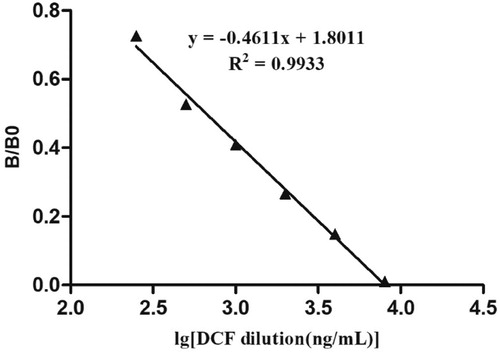
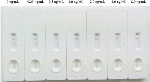
Figure 5. Standard DCF samples were tested using the ILFST and the T lines with the naked eyes.