RENEB/EURADOS field exercise 2019: robust dose estimation under outdoor conditions based on the dicentric chromosome assay

Figures & data

Figure 1. Irradiation setups and positions of samples for biological dosimetry. (A, C) setup of the first irradiation (phantoms P1 and P2), with samples P1-A (left hip) and P1-B (left shoulder) in red thermos flasks, samples P2-A (left hip) and P2-B (right hip) in black thermos flasks. (B, D) setup of the second irradiation (phantoms P3 and P4), with samples P3-A (left hip) and P3-B (left shoulder) in black, samples P4-A (left hip) and P4-B (right hip) in red thermos flasks. (E, F) RPL glass dosimeter reference doses measured outside the flasks. Red (hip) or yellow (shoulder) circles indicate the positions of flasks on the phantoms. Small blue circles indicate the position of the RPL reference glass dosimeters on the outside of the flasks. Missing doses are indicated by ‘NA’.

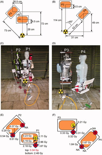
Table 1. RPL GD reference doses for tubes inside the thermos flasks.

Phantom	Code	Partner	RPL GDs inside thermos flasks (Dw, Gy)				Dose rate (Gy/h)
			GD-1 (Bottom)	GD-2 (Middle)	GD-3 (Top)	Median RPL dose
Close to source
1	P1-AI	PHE	2.22	1.79	2.02	2.02	2.02
1	P1-AII	IRSN	*	2.06	2.28	2.17	2.17
1	P1-AIII	BfS	3.11	1.52	1.57	1.54	1.54
1	P1-A(MIX)	BfS	2.13	1.91	1.46	1.91	1.91
1	P1-BI	PHE	0.09	0.09	0.15	0.09	0.09
1	P1-BII	IRSN	0.17	0.12	0.08	0.12	0.12
1	P1-BIII	BfS	0.17	0.14	0.10	0.14	0.14
1	P1-B(MIX)	BfS	0.20	0.17	0.18	0.18	0.18
Partly shielded
2	P2-A	PHE	0.38	0.37	0.41	0.38	0.38
2	P2-B	PHE	0.10	0.10	0.10	0.10	0.10
Distant
3	P3-AI	PHE	0.33	0.31	0.32	0.32	0.13
3	P3-AII	IRSN	0.26	0.22	0.31	0.26	0.10
3	P3-AIII	BfS	0.30	0.33	0.33	0.33	0.13
3	P3-B	IRSN	0.19	0.18	0.17	0.18	0.07
Lateral
4	P4-AI	PHE	1.36	1.38	1.83	1.38	0.55
4	P4-AII	IRSN	*	1.68	1.77	1.73	0.69
4	P4-AIII	BfS	1.31	1.20	*	1.25	0.50
4	P4-B	IRSN	0.06	*	0.04	0.05	0.02

Three tubes with 7 ml blood for each sample P1-A, P1-B, P3-A, P4-A and one tube for each sample P2-A, P2-B, P3-B and P4-B were equipped with three RPL GD reference dosimeters, each. One additional tube with 7 ml blood from P1-A and P1-B was mixed in a 50:50 ratio to simulate a heterogeneous exposure with two doses. The column ‘Partner’ indicates the laboratory that prepared the cell suspension. The cell suspension for sample P3-B was prepared by IRSN and sent to BfS for analysis. *Stands for missing dosimeter and dose in bold for outlier dose.

Figure 2. Calibration curves used by the participating laboratories. For dose estimation based on manual scoring, laboratories 6, 9, 14 and 16 used curves from (Barquinero et al. 1995). For dose estimation based on semi-automatic scoring, laboratory 16 used the curve described in (Vaurijoux et al. 2009). Curves based on manually or semi-automatically counted data are shown by solid or dashed lines, respectively.

Figure 3. RPL GD reference vs DCA dose estimates. (A) DCA dose estimates based on the assumption of an acute exposure. (B) DCA dose estimates based on the assumption of a protracted exposure considering the exposure times of each sample. Boxplots show the median and quartiles of the DCA dose estimates for each blood tube. Red dots indicate semi-automatically and blue dots manually scored DCA results. The DCA results of Lab17 (gray dots) were provided after the blind doses were distributed to the participants and are not considered in the evaluations. The RPL GD reference doses of each blood tube (2–3 replicates per tube) and the corresponding median values are shown by orange crosses and orange horizontal lines, respectively. Green rectangles show an interval of ±0.25 Gy around the median RPL GD reference dose of each tube.

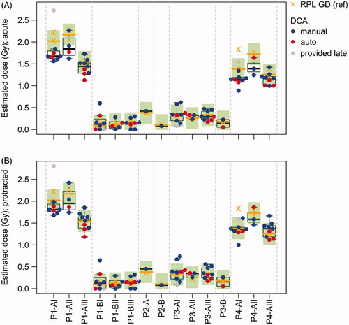
Table 2. DCA dose estimates from all participating laboratories (rows) for blood samples (columns) from all thermos flasks.

Lab	P1-A	P1-B	P2-A	P2-B	P3-A	P3-B	P4-A	P4-B
1^m	1.4^III	0.2^III			0.5^III	0.2	1.2^III
	(1.3; 1.6)	(0.0; 0.3)			(0.3; 0.6)	(0.1; 0.4)	(1.0; 1.3)
1^a	1.3^III	0.2^III			0.3^III	0.1	1.1^III
	(1.1; 1.5)	(0.0; 0.3)			(0.1; 0.5)	(0.0; 0.3)	(0.9; 1.3)
2^m	1.7^III	0.3^III			0.2^III		1.4^III
	(1.5; 2.0)	(0.1; 0.4)			(0.1; 0.3)		(1.2; 1.6)
2^a	1.1^III	0.1^III			0.2^III		1.0^III
	(0.9; 1.4)	(0.0; 0.3)			(0.0; 0.3)		(0.8; 1.2)
3^m	1.3^III	0.2^III			0.3^III		1.2^III
	(1.1; 1.5)	(0.0; 0.4)			(0.1; 0.5)		(1.0; 1.4)
4^m	1.6^III	0.0^III			0.5^III		1.2^III
	(1.3; 1.9)	(0.0; 0.3)			(0.2; 0.7)		(0.9; 1.4)
5^m	1.5^III	0.3^III			0.3^III		1.0^III
	(1.3; 1.7)	(0.1; 0.5)			(0.1; 0.5)		(0.8; 1.2)
6^m	1.5^III	0.0^III			0.4^III		1.3^III
	(1.2; 1.8)	(0.0; 0.2)			(0.2; 0.6)		(1.0; 1.5)
7^a	1.4^III	0.1^III			0.2^III		1.0^III	0.4
	(1.2; 1.6)	(0.0; 0.3)			(0.1; 0.4)		(0.8; 1.2)	(0.2; 0.6)
8^m	1.9^II	0.1^II			0.3^II		1.4^II
	(1.6; 2.2)	(0.0; 0.2)			(0.2; 0.6)		(1.1; 1.7)
9^m	1.6^II	0.0^II			0.2^II		1.2^II
	(1.4; 1.8)	(0.0; 0.2)			(0.0; 0.5)		(0.9; 1.6)
10^a	1.8^II	0.1^II			0.3^II		1.6^II
	(1.5; 2.1)	(0.0; 0.3)			(0.1; 0.6)		(1.4; 1.9)
11^m	2.3^II	0.3^II			0.3^I		0.9^I
	(2.1; 2.5)	(0.1; 0.5)			(0.1; 0.7)		(0.7; 1.1)
12^m	1.7^I	0.6^II			0.6^I		1.3^I
	(1.5; 1.9)	(0.4; 0.8)			(0.5; 0.8)		(1.2; 1.5)
13^m	1.6^I	0.2^II			0.6^I		1.2^I
	(1.4; 1.9)	(0.0; 0.4)			(0.4; 0.8)		(0.9; 1.4)
14^m	1.6^I	0.0^II			0.2^I		1.2^I
	(1.3; 1.8)	(0.0; 0.2)			(0.0; 0.4)		(1.0; 1.5)
15^m	1.7^I	0.1^II	0.4	0.1	0.1^I		1.1^I
	(1.5; 1.8)	(0.0; 0.3)	(0.3; 0.6)	(0.0; 0.2)	(0.0; 0.3)		(1.0; 1.3)
15^a	1.7^I	0.3^II			0.3^I		1.1^I
	(1.3; 2.0)	(0.0; 0.6)			(0.1; 0.6)		(0.8; 1.3)
16^m	1.8^I	0.1^II			0.3^I		1.1^I
	(1.6; 2.1)	(0.0; 0.3)			(0.2; 0.6)		(0.9; 1.4)
16^a	1.8^I	0.0^II			0.4^I		1.1^I
	(1.5; 2.1)	(0.0; 0.3)			(0.2; 0.6)		(0.9; 1.4)
(17^m)	2.7^I	0.0^II			0.1^I		1.5^I
	(2.3; 3.1)	(0.0; 0.2)			(0.0; 0.3)		(1.2; 1.9)

Doses are shown in Gy with corresponding 95% CIs in brackets. Dose estimates where the 95% CI included the median RPL GD reference dose are displayed in bold. The DCA results of Lab17 were provided after the blind doses were distributed to the participants and are not considered in the evaluations.

^aSemi automatic scoring; ^mmanual scoring; ^{I, II, III}Tube I, II or III.

Table 3. Percentage of DCA dose estimates (manual and semi-automatic scoring) for the ILC samples evaluated by the RENEB participants, including the median RPL GD reference dose in the 95% CI, within an interval of ±0.25 Gy or ±0.5 Gy or including 0 Gy in the estimated 95% CI.

	95% CI	±0.25 Gy	±0.5 Gy	0 Gy in 95% CI
P1-A
Manual & semi-auto	50%	40%	95%	0%
Manual	57%	50%	93%	0%
Semi-auto	33%	17%	100%	0%
P1-B
Manual & semi-auto	90%	95%	95%	70%
Manual	86%	93%	93%	71%
Semi-auto	100%	100%	100%	67%
P3-A
Manual & semi-auto	75%	90%	100%	5%
Manual	71%	86%	100%	7%
Semi-auto	83%	100%	100%	0%
P4-A
Manual & semi-auto	55%	65%	100%	0%
Manual	57%	64%	100%	0%
Semi-auto	50%	67%	100%	0%

Figure 4. Dispersion analysis for all samples analyzed by RENEB members. (A) Dispersion index for all samples. Dispersion index of 1 (horizontal orange line) indicates that the counts approximately follow a Poisson distribution. (B) U test statistic for all samples. For results with U > 1.96 the null hypothesis of equi-dispersion (Poisson assumption) can be rejected at the two-sided 5% significance level, indicating a heterogeneous exposure. Red dots indicate semi-automatically and blue dots manually scored results. The results of Lab17 (gray dots) were provided after the blind doses were distributed to the participants and are not considered in the evaluations. (C) Number of provided results with significant (p < .05, gray bar) or non-significant (black bar) U test.

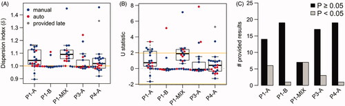
Table 4. Dose estimates based on the DCA for 50:50 mixture samples simulating a heterogeneous exposure.

	P1-MIX		P2-MIX		P3-MIX		P4-MIX
	D1	D2	D1	D2	D1	D2	D1	D2
Ref.	1.91	0.18	0.38	0.10	0.26	0.18	1.73	0.05
1^m	1.1 (100)				0.2 (100)
1^a	1.1 (100)				0.1 (100)
2^m	1.7 (66)	0.2 (34)
2^a	0.8 (100)
3^m	1.6 (34)	0 (66)
4^m	1.8 (63)	0 (37)
5^m	2.6	0
6^m	1.0 (100)
7^a	2.4 (41)	0.3 (59)
9^m	1.2 (100)
10^a	2.1 (41)	0 (59)					2.1 (25)	0 (75)
14^m	2.1 (67)	0 (33)
15^m	1.2 (100)		0.3 (100)
15^a	1.3 (100)

The row ‘Ref’. indicates the median RPL GD reference doses, the DCA dose estimates of the participating laboratories are displayed in the remaining rows. The columns D1 and D2 indicate the doses used for the 50:50 mixtures of a particular sample. The numbers indicate the estimated doses in Gy with the estimated percentage of cellls irradiated (in brackets) with dose D1 or D2.

^aSemi automatic scoring; ^mmanual scoring.

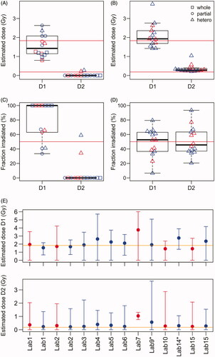
Figure 5. Dose estimates for the heterogeneous exposure simulated by sample P1-MIX. (A) Dose estimates provided by each laboratory. (B) Heterogeneous dose estimates re-calculated with the Biodose Tools software. (C) The estimated fraction of the body irradiated for the two doses as estimated by each laboratory. (D) The estimated fraction of the body irradiated for the two doses re-calculated with the Biodose Tools software. (E) Dose estimates for heterogeneous exposures with 95% confidence intervals estimated with the Biodose Tools software. In all sub-panels red color indicates semi-automatically and blue color manually scored results.

Barquinero JF, Barrios L, Caballín MR, Miró R, Ribas M, Subias A, Egozcue J. 1995. Establishment and validation of a dose-effect curve for gamma-rays by cytogenetic analysis. Mutat Res. 326(1):65–69.

 PubMed Web of Science ®Google Scholar

Vaurijoux A, Gruel G, Pouzoulet F, Gregoire E, Martin C, Roch-Lefevre S, Voisin P, Voisin P, Roy L. 2009. Strategy for population triage based on dicentric analysis. Radiat Res. 171(5):541–548.

 PubMed Web of Science ®Google Scholar