The colonization of an irradiated environment: the case of microbial biofilm in a nuclear reactor

Figures & data

Figure 1. (A) Side view of the JSI TRIGA Mark II research reactor. The ladder with sampling slides was positioned close to wall on the left-hand side of this schematic, indicated by a full black vertical line. See Figure 2 for photograph of the glass slides. (B) Schematic figure of the JSI TRIGA reactor core. Channel F26 is located in the outer ring of JSI TRIGA core (black arrow).

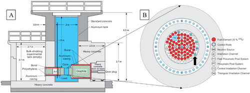
Figure 2. JSI TRIGA research reactor pool with ladder and attached glass slides. To the left of the ladder is the reactor core. Biofilm growing on the wall itself can be observed. Red arrows indicate position of the biofilm sampling glass slides. Photograph taken during glass-slide deployments on the 30 December 2014. See Figure 1 caption for placement information.

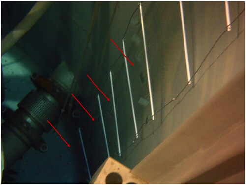
Table 1. Measured doses by depth at constant reactor power (1 kW).

Depth (m)	Background dose (mSv/h)	Dose at 1 kW (mSv/h)
1	–	0.1
2	–	0.23
3	<0.1	4.6
4	0.51	143
5	48.1	2400
6	12.4	790

Table 2. Chemical conditions on the 16 January 2014, at the beginning and at the end of first the biofilm sampling.

t [GMT + 1]	09:00:00
pH	5.63
TDS	4.10	ppm
Conductivity	6.54	µS
ORP	140	mV
T	23.3	°C
Total alkalinity	0.026	mM
t [GMT + 1]	13:15:00
pH	5.70
TDS	2.33	ppm
Conductivity	3.68	µS
ORP	157	mV
T	19.0	°C

Long-term conditions do not change much, except the increase in the water temperature during reactor operation. On the sampling day, however, total dissolved solids, conductivity and oxidation reduction potential values show the quality of the water improved after the scrubbed biofilm has been removed by filtering.

Table 3. Stable isotope analysis of reactor water and biofilm.

	δ^15N	wt.%N	C/N	δ^13C	wt.%C
Water	<LOD	–	<LOD	<LOD	–
Biofilm	−1.5	7.7	–	−31	43.4
	−2.3	8.3	–	−30	40.1
			–	−30.7	46.1
Average	−1.9	8	5.4	−30.6	43.2
µg/L	TOC	TOC (0.45 µm)	DOC	DOC (0.45 µm)	DIC	DIC (0.45 µm)
Water	<LOD	<LOD	0.17	0.15	<LOD	<LOD

See text for discussion on results.

Table 4. Results of ICP-MS screening of reactor biofilm.

ICP light elements		(µg/g) dw
Fe	Ca	K	Na	Mg	Ni
4406.2	Interference with Ar	269.6	−203.2	330.3	50.4
ICP heavy elements		(µg/g) dw
Sb	As	Cu	Zn	Mn	Cd	Co
1.3	1.2	214.6	99.0	24.7	6.4	6.7
Cr	Mo	Au	Se	Pb	Ag
218.0	28.4	0.2	1.0	38.4	3.6

The investigated metals have a biogenic role, but can be toxic in higher concentrations. The ICP-MS analysis of water showed almost no presence of the same investigated elements. The extremely high Al content is not surprising and is expected to be abundant, since it is construction element of the reactor tank wall.

Table 5. Visual characteristics of pure cultures chosen for 16S rDNA Sanger sequencing.

Depth/ sample	Diameter (mm)	Texture	Color	Edge	Genus/species
1.5 m	2–3	Creamy	Grey	Round, entire	B. flexus
2 m	2–4	Compact	Bright yellow	Entire	Frigoribacterium sp.
2.5 m	2–4	Creamy	Light pink	Entire	Arthrobacter sp.
3 m	3–4	Creamy	Grey	Round entire	B. flexus

Table 6. Overview of samples for metagenomic 16S rDNA sequencing.

Sample number	Depth	Genus/species	Colony description	Sampling date
1	2 m	Frigoribacterium sp.	Pure culture, yellow	26 May 2014
2	2.5 m	Arthrobacter sp.	Pure culture, pink	26 May 2014
3	3 m	Bacillus flexus	Pure culture, γ irradiated	26 May 2014
4	4 m	N/A	Native sample	30 December 2014
5	3 m	N/A	Native sample	30 December 2014
6	5.5 m	Sphingomonas sp.	Pure culture, white	05 August 2014
7	5.5 m	Variovorax sp.	Pure culture, yellow	05 August 2014
8	5.5 m	Bacillus flexus	Pure culture, grey	05 August 2014
9	5.5 m 1 week	N/A	Native sample	06 January 2015
10	5.5 m 2 week	N/A	Native sample	13 January 2015

Not all the samples are highlighted in the text. See Supplementary Tables S1 and S2 for detailed information.

Figure 3. Epifluorescence micrographs of native biofilm under excitation with UV illumination corresponding to autofluorescence of chlorophyll a. A 3D composite image (not shown) showed the chlorophyll was distributed throughout the biofilm, meaning there was no spatial segregation of the phototrophs.

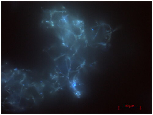
Figure 4. Colony of B. flexus, after irradiation with γ + n⁰. Agglomeration in sphere-like structure was not anticipated. No further growth was observed. Photograph taken on 13 November 2014.

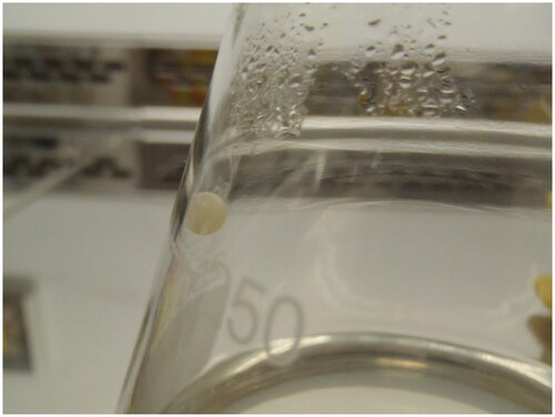
Figure 5. Scanning electron micrograph showing individual bacterial cells on smooth (A) and frosted (B) surface of glass slides at depth of 5.5 m and clusters of bacterial cells on smooth (C) and frosted (D) surface of slide at depth of 3 m. Black bar denotes 1 μm on images A, B, C, and 10 μm on image D. Images were taken with field-emission scanning electron microscope.

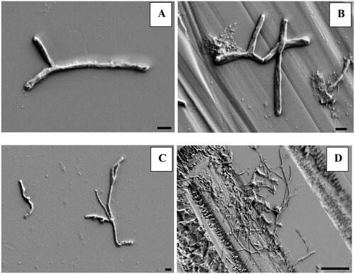
Figure 6. Representation of 1-week (sample 9), 2-week (sample 10) and 4 m depth microbial communities’ diversity (sample 4) by 16S rDNA amplicon sequencing. Only genera with more than 1% abundance are shown and ‘other’ refers to the detected genera with lower abundance (see the interactive supplementary table S3 for full description). See discussion for more info.

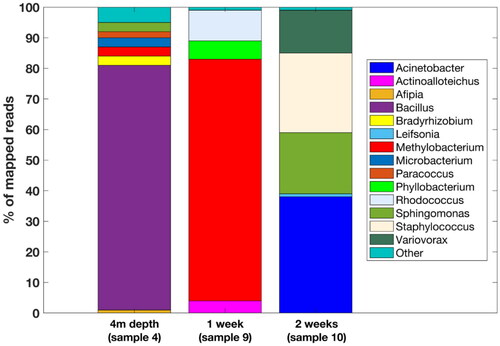
Table 7. Doses per glass slide.

Depth (m)	Background dose (mSv/h)	Dose at 1 kW (mSv/h)	Received dose (Gy)
			1 week slides – 251 kWh	2 weeks slides – 282 kWh	3 weeks slides – 6250 kWh	8 weeks slides – 15,900 kWh
2.5	0	2.42	0.606	0.681	15.1	38.4
3.5	0.26	73.8	18.6	20.9	431	1170
4	0.51	143	36.0	40.5	894	2270
5	48.1	2400	611	693	15,000	38,200

Since the reactor does not operate regularly, received doses to the bacteria are not proportional to the time spent inside reactor pool. In order to calculate received doses, a reactor log is needed. Therefore, we can calculate released heat. Using that data and results from Table 1, we can calculate the exact dose per slide that was placed inside reactor pool.