Fireside corrosion and deposition on heat exchangers in biomass combustion systems

Figures & data

Figure 1. Schematic diagram of corrosion coupons used for the tests [13,14].

Table 1. Nominal composition for selected alloys (wt%) [22,23].

Material	C	Cr	Ni	Mo	Mn	V	Nb	Fe
TP347HFG	0.07	18	10	-	2	-	1	Balance
T91	0.14	9	0.4	1	0.5	0.25	0.1	Balance

Figure 2. Schematic diagram of corrosion furnace used for the test.

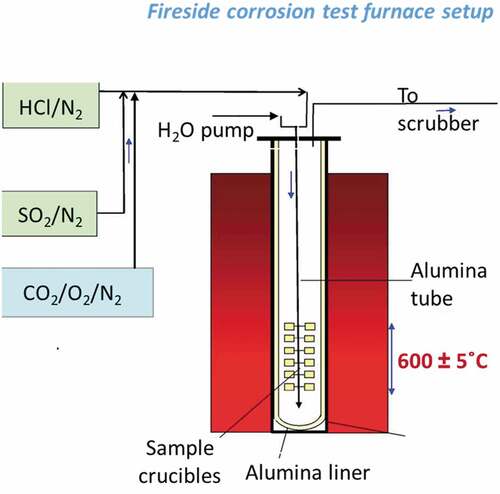
Table 2. Molar composition of the three different deposits used in the test.

Deposit	KCl	K2SO4		Na2SO4	CaSO4
	Concentration (mole %)
D1	30	20	20			30
D6	71	29
D8	67	33

Table 3. Composition of the simulated APR combustion gas environment.

Gas composition	N2	O2	CO2	SO2	HCl	H2O
Mol %	70.3	6.2	11.8	96.0 vol. ppm	53.0 vol. ppm	11.6

Figure 3. Schematic representation of the dimensional metrology process. The analysis consists of different steps 1) measuring the samples before exposure, 2) samples’ mounting in resin, 3) imaging of samples’ perimeters, 4) selecting of points at the metal surface and for internal damage, 5) comparing samples with pre-exposure measurements and reference samples, 6) subtracting the environmental effect by comparison to a sample exposed to the same environment without deposit, 7) plotting the resulting change in metal against location and 8) re-ordering the data based on cumulative probability [23,25].

Figure 4. Fireside distribution plot for metal change after a) 200 h; c) 500 h, e) 1000 h exposure; and sound metal change after b) 200 h, d) 500 h and f) 1000 h exposure, for both alloys and all three deposits.

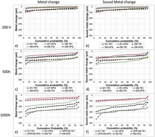
Figure 5. Time distribution for the median metal and sound metal change. The bar chart shows the behaviour of the different alloys and different deposits. The error bars in the chart represent the maximum and minimum change of the different distributions.

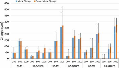
Figure 6. Backscattered images of the two different alloy and different deposits.

Figure 7. Backscattered images of T91-D1 and 347HFG-D1 on the left-hand side with respective EDX maps after 500 h exposure.

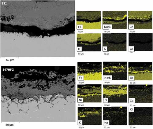
Figure 8. Backscattered images of T91-D6 and 347HFG-D6 on the left-hand side with respective EDX maps after 500 h exposure.

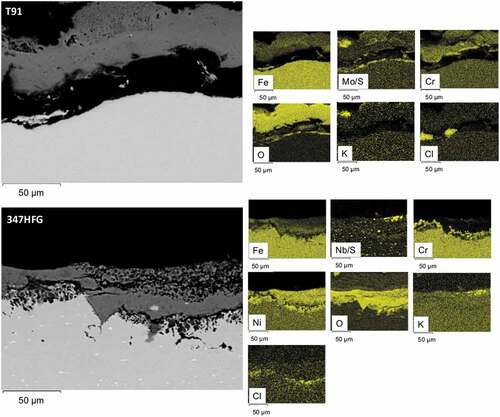
Figure 9. Backscattered images of T91-D8 and 347HFG-D8 on the left-hand side with respective EDX maps after 500 h exposure.

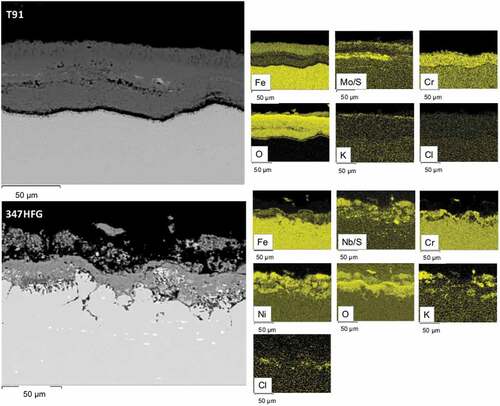
Figure 10. Backscattered image of 347HFG-D6 after 1000 h exposure, showing Cl attack mode.

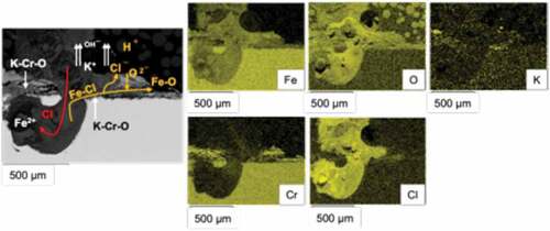
Figure 11. Backscattered image of 347HFG-D1 after 500 h exposure showing K-Na possible location.

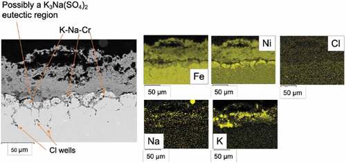
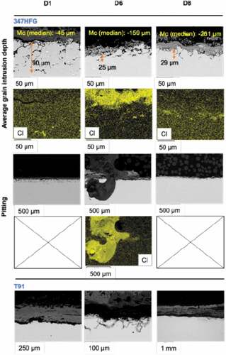
Figure 12. Backscattered images and EDX maps for 347HFG with different deposits showing median penetration depth. Bottom figures represent T91 samples with different deposits after 500 h exposure.

Michelsen HP, Frandsen F, Dam-Johansen K, et al. Deposition and high temperature corrosion in a 10 MW straw fired boiler. Fuel Process Technol. 1998;54(1–3):95–108.

 Web of Science ®Google Scholar

Mori S, Pidcock A, Sumner J, et al. Fireside corrosion of heat exchanger materials for advanced solid fuel fired power plants. Oxid Met. 2022;97(3–4):281–306.

 Web of Science ®Google Scholar

He J, Xiong W, Zhang W, et al. Study on the high-temperature corrosion behavior of superheater steels of biomass-fired boiler in molten alkali salts’ mixtures. Adv Mech Eng. 2016;8(11):1687814016678163.

 Web of Science ®Google Scholar

Global Steel & Alloys. ASTM A213/ASME SA213 T2, T11, T12, T22, T91, T92 chemical composition and mechanical properties 2021.

 Google Scholar

Hussain T, Syed AU, Simms NJ. Fireside corrosion of superheater materials in coal/biomass co-fired advanced power plants. Oxid Met. 2013;80(5–6):529–540.

 Web of Science ®Google Scholar