Figures & data
Figure 1. Left – pressure vessel in open split-furnace, just after EPD connections have been completed. Right – routing and conversion of high temperature (HT) wiring to room temperature (RT) cabling.
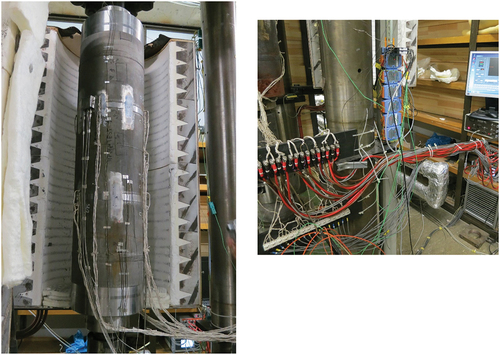
Figure 2. Left – pre-soldered stud connections ahead of installation, Mid – modified stud gun head. Right – rapidly welded stud array (minus wiring).
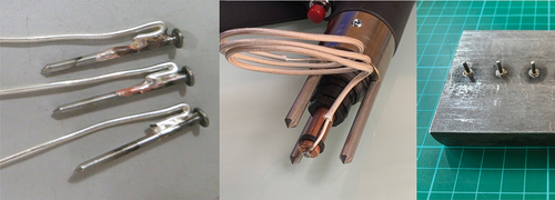
Figure 3. Top – as made stud/wire connections ahead of creep test. Bottom – after 10k hour test duration – note unoxidised silver wire.
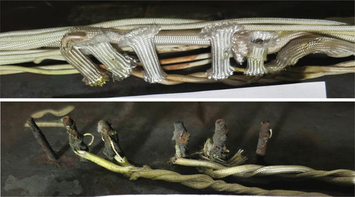
Figure 4. Left – Stud connections after installation on horizontal vessel. Right – close up of a set of 6 studs, the outer two for the excitation current and two inner pairs for the signal from each HAZ.
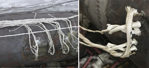
Figure 5. Schematic of a full AC/DC EPD system in a condition monitoring role. The local junction between RT (copper) and HT (silver) wiring is undertaken as soon as the HT wiring exits the hot zone.
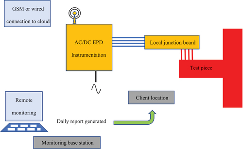
Figure 6. DCPD over time (4 months) – initial rise to level due to heat up of furnace, with subsequent transients due to temperature control issues with furnace. The large swings far exceed that due to incipient damage by orders of magnitude.
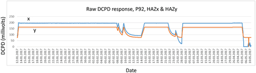
Figure 7. Processed DCPD over time (2 months). Transients (any data 10% above or below running average) were removed, and data auto-scaled to reveal random signal noise. Slow but steady rise due to possible incipient damage then emerges.
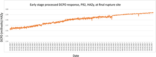
Figure 8. Raw DCPD over time (2 months) as final failure occurs – steady rise overtaken by exponential rise as crack propagates. Shielding effect on adjacent HAZ means complimentary DCPD drops.
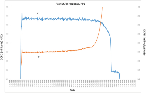
Figure 9. Raw ACPD over time (2 months) at final failure – steady drop overtaken by exponential rise as crack propagates. Shielding effect on adjacent HAZ means complimentary ACPD drops. Transients not removed.
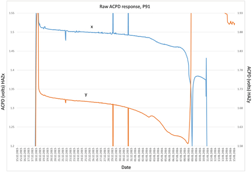
Figure 10. Top – DCPD line-scans along interrupted test specimens (bottom). Life fraction estimated to be less than 20% for these specimens over virgin material (also shown). No convincing trends can be detected.
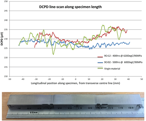
Figure 11. Top – ACPD line-scans along interrupted test specimens. Definite peaks are detectable, with central peak corresponding to location of HAZ. Further peaks (multiple passes?) can also be detected.
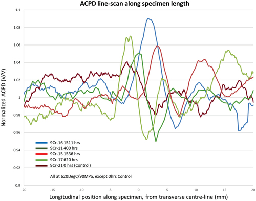
Figure 12. Variation in ACPD peak height (main peak) with life fraction (estimated).
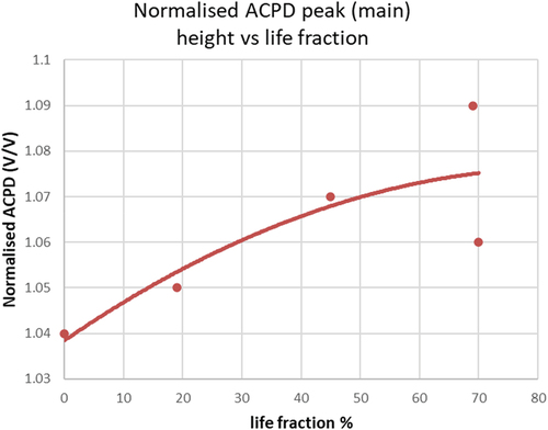
Figure 13. Variation in average ACPD (across main part of specimen) with life fraction (estimated).
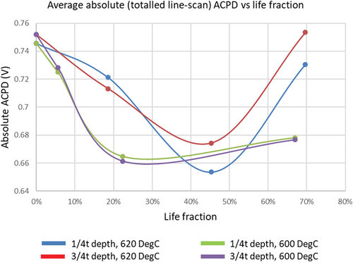
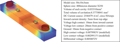
Figure 14. (a) LHS, meshed CAD model of test specimen, (b) RHS, modelled current distribution. Current is input/extracted via the two large posts on top surface. Voltages ‘read’ off on the inner two posts. DCPD is the differential value between inner contacts. Modelling parameters are given alongside.
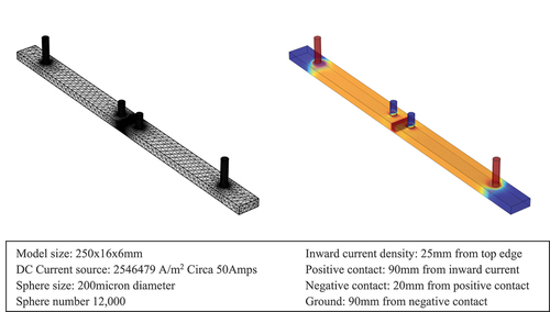
Figure 15. Simplified and shortened ‘reference’ specimen showing identical modelled current flow. Modelling parameters are given alongside.
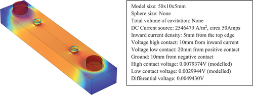
Figure 16. Cavity creation methodology, left to right, a single layer, a cube of layers, an array of cubes.
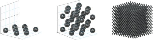
Figure 17. (a) LHS, modelled current flow in a cavitated specimen, for a cavity radius of 100 microns, and a cavity number of 8000, (B) RHS, close up of the cavitated area showing the banding in the current flow, characteristic of the model and the way in which the cavities are stacked.
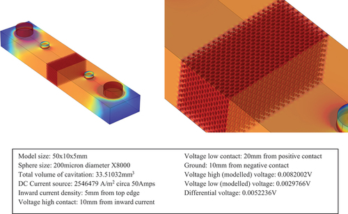
Figure 18. Plot of calculated DCPD against % total cavitation (% porosity) for the constant cavity radius (variable cavity count) model. Equation fit given on plot.
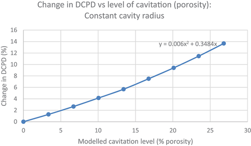
Table 1. Tabulated values of the modelled DCPD voltages and cavity volumes for a model with cavity size at 100 micron radius, but with variable cavity count.
Figure 19. Modelled current flow in a cavitated specimen, for the constant cavity number model, (variable cavity size). 250 cavities shown, of 200 micron radius.