
Figures & data
Figure 1. Correlation between share education level and log population in Core-Cities; China 2000, 2010. Source: calculations based on Chinese census of population, 2000 and 2010; see the main text for details.
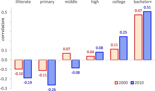
Figure 2. Initial population size and change in education level in Core-Cities; China 2000–2010. Source: Calculations based on Chinese census of population, 2000 and 2010; log population in 2000 on horizontal axis; change in education share from 2000 to 2010 (in percentage points); dotted line is a trendline; 251 Core-Cities included; see main text for details.
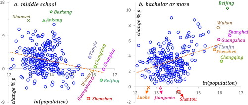
Figure 3. Selected skill sorting as measured by education level in Core-Cities; China, 2010. Source: Chinese census of population, 2010; vertical axis depicts the log of the number of people with a certain education level living in the city; see the main text for details.
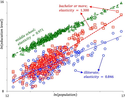
Table 1. Summary of administrative division at prefectural, Extended-City and Core-City levels
Figure 4. Yancheng prefecture; Jiangsu province, China, 2010.
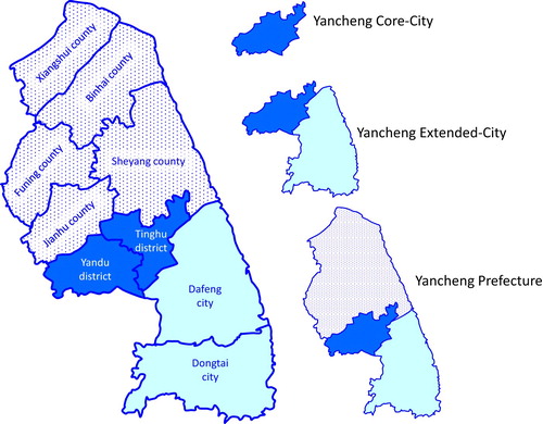
Figure 5. Core-Cities and Extended-Cities; rank-size distribution, 2010. The panels depict the upper (median and above) rank-size distributions for core-cities (panel a) and extended-cities (panel b); see main text for definitions; dashed lines are trendlines; slope is –1.4314 and –1.5684, share of variance explained is 98.4% and 95.5%, with 142 and 158 observations for core-cities and extended-cities, respectively.
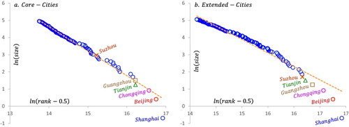
Table 2. Population shares of skill group by educational attainment in 2000 and 2010 (%).
Table 3. Average education of employment and population share in each sector.
Table 4. Average education of employment and population share in each occupation.
Table 5. Population elasticities of educational groups.
Figure 6. Education population elasticities and skill intensity (in years of schooling). The size of the bubble measures the size of each educational level; the fitted lines are weighted by population shares; the vertical axis does not start at zero; see for categories.
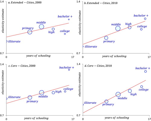
Table 6. Hypothesis 1 elasticity test: large locations are more education-skill intensive.
Figure 7. Pairwise comparison of six educational attainment levels. The bins are 2; 4; 10; 30; 90; individual; the associated number of pairs are 15; 90; 675; 6525; 60,075; at least 548,775; the dashed lines indicate the upper and lower limits of a 95% confidence interval of tossing a fair coin; the interval is exact up to 15 pairs and based on the Central Limit Theorem otherwise; each panel is based on more than one million bilateral comparisons, the whole figure on about five million bilateral comparisons. Note if the condition holds; value = 1 and if not; value = 0; if the outcome would be random the average value would be 0.5.
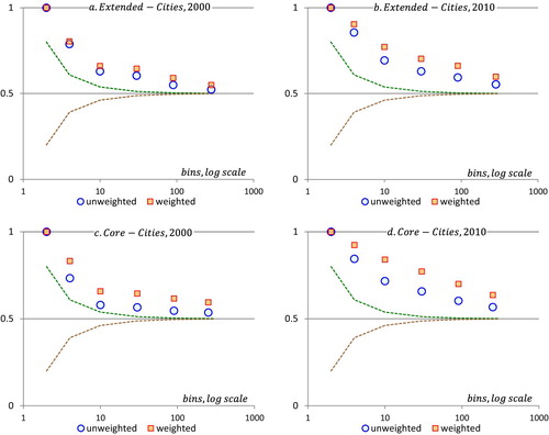
Figure 8. Sector population elasticities and skill intensities. The size of the bubble measures the size of sectors; the fitted lines are weighted by population shares; the vertical axis does not start at zero.
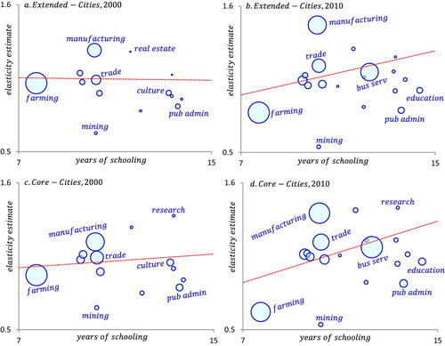
Table 7. Hypothesis 1 elasticity test: large locations have more skill intensive sectors/occupations.
Figure 9. Occupation population elasticities and skill intensities. The size of the bubble measures the size of occupations; the fitted lines are weighted by population shares; the vertical axis does not start at zero; technical = technical personnel.
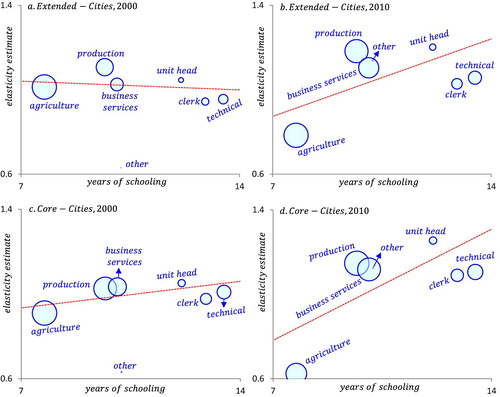
Figure 10. Pairwise comparison of sectors and occupations for Cities. The bins are 2; 4; 10; 30; 90; individual; the associated number of pairs for occupations are 21; 126; 945; 9135; 84,105; at least 658,875; the associated number of pairs for sectors are 171; 1026; 7695; 74,3855; 684,855; at least 3.3 million; the dashed lines indicate the upper and lower limits of a 95% confidence interval of tossing a fair coin; the interval is exact for 21 pairs and based on the Central Limit Theorem otherwise; each panel is based on more than 1.5 million bilateral comparisons, the whole figure on 25.5 million bilateral comparisons; there are 15 sectors in 2000 and 19 sectors in 2010; there are 7 sectors in both years. Note if the condition holds; value = 1 and if not; value = 0; if the outcome would be random the average value would be 0.5.
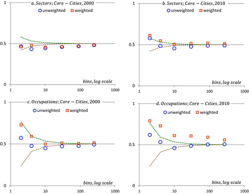
Table A1. Full name and short name of sector and occupation.