Conventional and geometric morphometric studies of valve ultrastructural variation in two closely related Cyclotella species (Bacillariophyta)

Figures & data

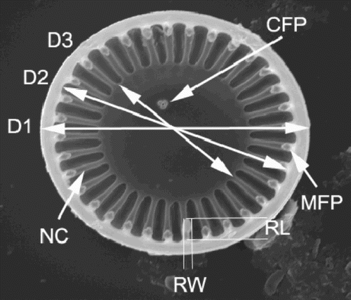
Fig. 1. Variables used for the conventional morphometric analyses, illustrated on a C. meneghiniana valve. D1 – valve diameter; D2 – valve diameter measured between the inner edges of the mantle (i.e., D1 minus twice the mantle thickness); D3 – diameter of the central area; RW – width of the rimoportula; RL – length of the rimoportula; NC – number of costae; MFP – number of marginal fultoportulae; CFP – number of central fultoportulae.

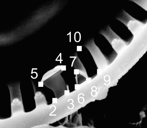
Fig. 2. Positions of landmarks 2 to 9 used for the geometric morphometric analyses shown on a valve from the ‘ambiguous’ morph. Landmark 1, the midpoint of the valve is not shown here. Table 1 describes positioning of the landmarks.

Table 1 . Landmark points recorded for the geometric morphometric analyses. Their position is described on a valve, the RP of which was oriented towards the bottom of the image. See also Fig. 2

Number	Description
1	The centre of the valve
2	The distal right corner of the alveolus at the left of the rimoportula (RP)
3	The distal left corner of the alveolus at the right of the RP
4	The end of the RP looking towards the upper right corner of the image
5	The other end of the RP head
6	The distal right corner of the alveolus at the right of the RP
7	The tip of the marginal FP at the first costa to the right of the RP
8	The distal left corner of the second alveolus on the right-hand side of the RP
9	The distal right corner of the same alveolus
10	The midpoint of the proximal edge of the same alveolus

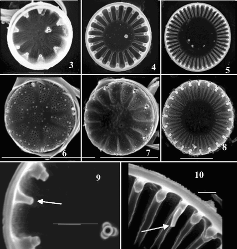
Figs 3–10. Scanning electron micrographs of valves from Cyclotella meneghiniana cultures. Figs 3–5. Valve interiors. Figs 6–8. Valve exteriors over the size range. Figs 9–10, Detail of interior margins showing rimoportulae (arrows) in an extremely small (Fig. 9) and a larger (Fig. 10) valve. Scale bars represent 5 µm (Figs 3–8) and 1 µm (Figs 9, 10).

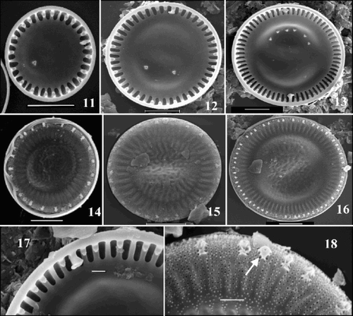
Figs 11–18. SEM images of valves of the ‘ambiguous’ morph of Cyclotella scaldensis. Figs 11–13. Valve interiors. Figs 14–16. Valve exteriors over the size range. Fig. 17. Interior margin showing rimoportula. Fig. 18. Exterior margin showing process openings; RP opening is marked by an arrow. Scale bars represent 5 µm (Figs 11–16) and 1 µm (Figs 17, 18).

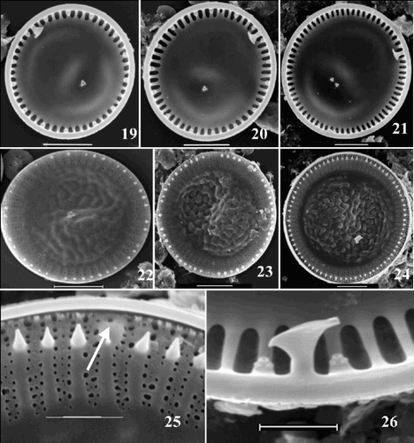
Figs 19–26. SEM images of valves of the ‘extreme’ morph of Cyclotella scaldensis. Figs 19–21. Valve interiors. Figs 22–24. Valve exteriors over the size range. Fig. 25. Exterior margin, showing process openings; RP opening marked by an arrow. Fig. 26. Interior margin with RP and two neighbouring FPs. Scale bars represent 5 µm (Figs 19–24) and 2 µm (Figs 25, 26).

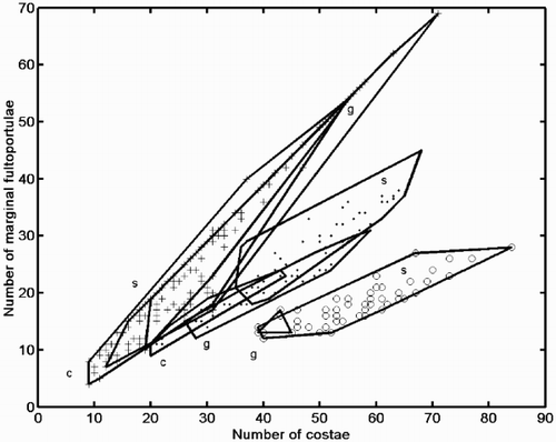
Fig. 27. Scatter plot of number of costae (NC) against number of marginal fultoportulae (MFP). Group outliers are connected by lines. (+ = C. meneghiniana, = ‘ambiguous’ morph of C. scaldensis, ○ = ‘extreme’ morph of C. scaldensis. c = cultures, g = field samples from the River Geeste, s = field samples from the river Schelde.)

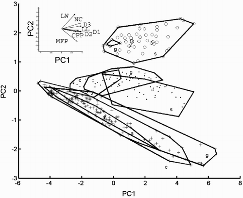
Fig. 28. Scatter plot on the first two principal component axes of the conventional morphometric dataset. Group outliers are connected by lines. (+ = C. meneghiniana, = ‘ambiguous’, ○ = ‘extreme’ morph of C. scaldensis. c = cultures, g = field samples from the River Geeste, s = field samples from the river Schelde.) Vector correlations of the original variables with the first two principal components are shown in the upper left hand corner.

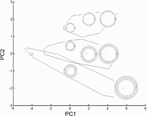
Fig. 29. Reconstructed morphologies of some points in the plane of the first two principal component axes (data shown in Fig. 28). Group outliers of the three morphs are shown. Morphologies were ‘reconstructed’ by projecting PCA scores back into the coordinate system of the original variables and drawing diagrams based on the resulting values (see ‘Materials and methods’ for details). The diagrams are drawn at the same scale. The morphologies shown correspond to PCA scores (−4, 0), (0, −1), (0, 0.5), (0, 1.5), (2, 0), (2, 2), (4, 0), (4, 2) and (6, −2).

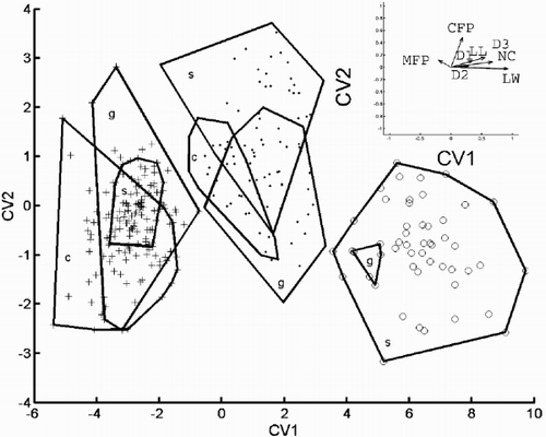
Fig. 30. Canonical variate analysis of the conventional morphometric dataset. Canonical variate scores calculated by grouping the specimens according to morph. (+ = C. meneghiniana, = ‘ambiguous’, ○ = ‘extreme’ morph of C. scaldensis; c = cultures, g = field samples from the River Geeste, s = field samples from the river Schelde.) Group outliers are connected by lines. Vector correlations of the canonical variates with the eight original variables are shown in the upper right hand corner.

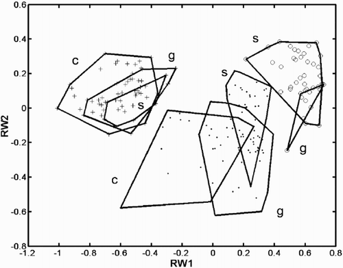
Fig. 31. Relative warp analysis with α = −1, small scale differences weighted more than global ones. Scores of specimens on the first two relative warp axes. Group outliers are connected by lines. (+ = C. meneghiniana, = ‘ambiguous’, ○ = ‘extreme’ morph of C. scaldensis; c = cultures, g = field samples from the River Geeste, s = field samples from the river Schelde.)

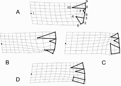
Fig. 32. Landmark configurations corresponding to some points of Fig. 31 depicted as deformations from the mean configuration (the origin of the coordinate system in Fig. 31). Figure 32A corresponds to the point (0, 0.5) of the coordinate system, Fig. 32B to (−0.5, 0), Fig. 32C to (0.5, 0), and Fig. 32D to (0, −0.5). The points connected by thick lines represent the landmark points shown in Fig. 2, but the diagrams are rotated approximately 90° anti-clockwise compared to Fig. 2.

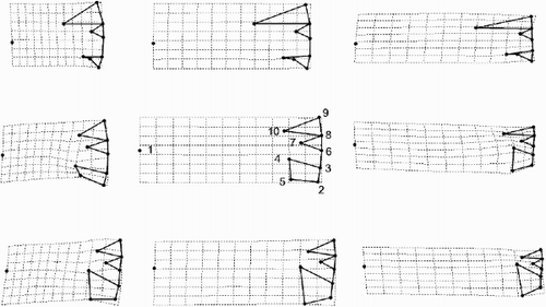
Fig. 33. Patterns of allometric valve shape change in the three morphs with size as calculated from a linear regression of the partial warp scores on the logarithm of valve diameter. Landmarks (see Fig. 2 to link them to the anatomic features of the valve interior) are connected by thick lines but the diagrams are rotated approximately 90° anti-clockwise compared to Fig. 2. The landmark configurations predicted by the regression for three different diameters (D1 = 8, 16 and 24 µm, respectively) in the three morphs are shown in the columns and the different taxa by rows. Row 1 = Cyclotella meneghiniana, row 2 = ‘ambiguous’ morph of C. scaldensis and row 3 = ‘extreme’ morph of Cyclotella scaldensis.