Optimizing the biomass balance of macroalgae and sea urchins in kelp beds by removing the urchins

Figures & data

Fig. 1. Schematic diagram of ocean currents and study sites around Hokkaido, Japan. The red and blue arrows indicate warm and cold water currents, respectively. TSC, Tsushima warm current; TGC, Tsugaru warm current; SC, Soya warm current; OC, Oyashio cold current (Kurile current); LC, Liman cold current; ESC, East Sakhalin current. Sea urchin removal experiments were conducted in the southwestern (SW; Kaminokuni), northwestern (NW; Rishirifuji) and northeastern (NE; Esashi) coastal regions of Hokkaido. Oceanographic surveys were conducted at Kaminokuni, Hiyama-Esashi, Setana, Rishiri, Rishirifuji, and Monbetsu coastal regions. Shaded areas along the coastline indicate the occurrence of sea urchin barrens.

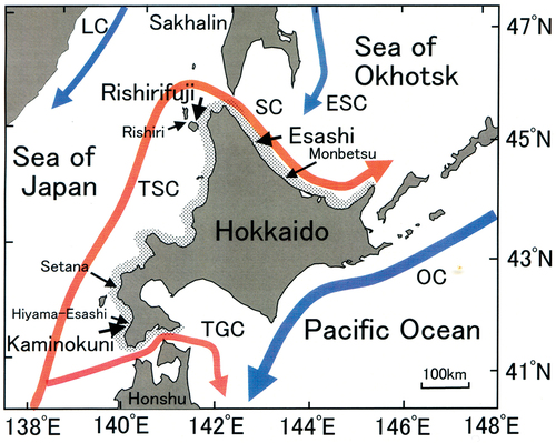
Fig. 2. A photograph of sea urchin removal performed by a diver in the southwestern (SW; Kaminokuni) coastal region of Hokkaido.

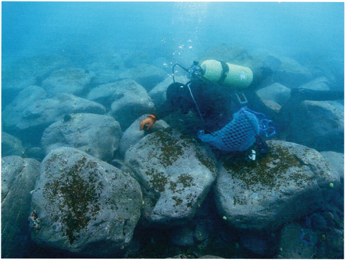
Fig. 3. Monthly fluctuation in mean seawater temperatures of surface water for 10 days (mean ± standard error) in the coastal regions of southwest (SW, neighbouring Hiyama-Esashi 2001–2005; Kaminokuni 2001–2010, n = 8–10), northwest (NW; Rishirifuji 1991–1998, n = 8) and northeast (NE; Esashi 1995–2000, March–November n = 5, December n = 2). Seawater temperature data in NE from January to early mid-March were not measured because of the sea-ice berthing period.

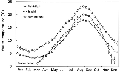
Fig. 4. Monthly fluctuation in mean inorganic nutrient concentrations (NO₃-N, upper; PO₄-P, lower) of surface seawater (mean ± standard error) in the coastal regions of southwestern (SW; Setana 1999–2006, n = 4–8), northwestern (NW; Rishirifuji 1999–2006, n = 5–8) and northeastern sites (NE; Monbetsu 2007–2013, n = 7). ND, no data.

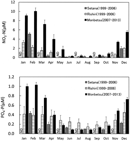
Fig. 5. Effects of sea urchin removal (SUR) on the biomass of macroalgae and sea urchins (g wet weight m⁻², mean ± standard error) in the southwestern site (SW, Kaminokuni) from September 2010 to May 2013 (SUR, n = 5–12; control, n = 4).

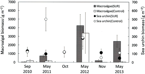
Fig. 6. Effects of sea urchin removal (SUR) on the biomass of macroalgae and sea urchins (g wet weight m⁻², mean ± standard error) in the northwestern site (NW, Rishirifuji) of Hokkaido from September 1989 to September 1993 (SUR, n = 2–9; control, n = 3). ND, no data (September 1989).

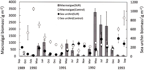
Fig. 7. Effects of sea urchin removal (SUR) on the biomass of macroalgae and sea urchins (g wet weight m⁻², mean ± standard error) in the northeastern site (NE, Esashi) of Hokkaido from May 1989 to June 1992 (SUR, n = 3–17; control, n = 2–5). ND, no data (September 1989, April 1991, May 1991 and July 1991).

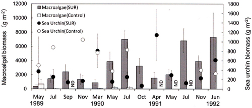
Table 1. Comparisons of seaweed biomass (g wet weight m⁻² ± SE) among study sites (SW, Kaminokuni 2009–2013; NW, Rishirifuji 1989–1992; NE, Esashi 1989–1991) with and without sea urchin removals (SUR).

	Kaminokui		Rishirifuji		Esashi
	SUR	Control	SUR	Control	SUR	Control
Chlorophyceae
Cladophora opaca	0.3 ± 0.3	1.2 ± 0.9
Cladophora sp.	+				+
Enteromorpha sp.					+
Monostroma nitidum			1.7 ± 1.0	0.7 ± 0.5	+
Ulva pertusa	19.0 ± 19.0		84.5 ± 22.7	1.0 ± 0.5	8.8 ± 4.8	0.3 ± 0.3
Phaeophyceae
Agarum clathratum			0.1 ± 0.1	0.2 ± 0.2
Colpomenia sinuosa	0.7 ± 0.7
Costaria costata*	17.7 ± 14.6	12.1 ± 9.4	7.1 ± 3.6	+	11.4 ± 6.5	18.5 ± 16.5
Dactylosiphon bullosus	0.1 ± 0.1		+	+	+
Desmarestia viridis	38.1 ± 32.0	0.9 ± 0.6	2.1 ± 1.4	+	+
Dictyota dichotoma	3.4 ± 2.2		10.7 ± 6.6	0.1 ± 0.1
Dilophus okamurae	0.7 ± 0.5	2.3 ± 1.7	1.5 ± 1.3	+
Petalonia fascia	5.9 ± 3.3	44.6 ± 34.6	13.0 ± 7.4	16.7 ± 16.7	2.0 ± 1.4	7.5 ± 7.1
Punctaria latifolia			11.2 ± 11.2	+
Saccharina japonica var. ochotensis*			378.6 ± 175.2	0.3 ± 0.3	2644.1 ± 577.0	518.3 ± 237.9
Saccharina japonica var. religiosa*	318.3 ± 298.7	480.8 ± 372.1
Sargassum confusum*	11.2 ± 11.2		+	0.2 ± 0.2
Sargassum miyabei*			+	+
Sargassum siliquastrum*	15.6 ± 10.9
Scytosiphon lomentaria	23.1 ± 14.8	2.8 ± 1.4	11.2 ± 5.5	2.1 ± 2.1
Stephanocystis hakodatensis*	38.9 ± 38.9
Undaria pinnatifida*	183.4 ± 95.9	0.1 ± 0.1	27.8 ± 17.9	+
Rhodophyta
Bonnemaisonia hamifera	0.3 ± 0.3	0.9 ± 0.7	0.2 ± 0.2	0.7 ± 0.7
Bossiella sp.	+		0.1 ± 0.1	0.1 ± 0.1	+
Ceramium japonicum	+
Ceramium kondoi	16.7 ± 14.2		0.3 ± 0.3	+	0.4 ± 0.4	2.2 ± 2.2
Chondria crassicaulis	0.1 ± 0.1		+	+
Chondrus armatus					0.9 ± 0.9
Chondrus ocellatus					0.1 ± 0.1
Chondrus sp.	0.8 ± 0.6
Chordaria flagelliformis					1.0 ± 0.7
Chrysymenia wrightii	0.1 ± 0.1
Congregatocarpus kurilensis			+	+
Corallina pilulifera	0.6 ± 0.6		0.1 ± 0.1	+
Cumathamnion serrulatum	5.1 ± 4.9		28.8 ± 12.8	1.0 ± 1.0
Dasya sessilis	0.3 ± 0.3
Dumontia contorta					+
Fushitsunagia catenata	0.7 ± 0.7	+
Gelidium elegans			0.2 ± 0.2	+
Gelidium vagum	0.4 ± 0.4	0.2 ± 0.1
Grateloupia turuturu					+
Gymnogongrus flabelliformis			+	0.7 ± 0.7
Gymnogongrus flabelliformis	0.3 ± 0.3
Laurencia nipponica	0.4 ± 0.4				0.3 ± 0.4	+
Laurencia okamurae	0.5 ± 0.5
Laurencia pinnata	+
Laurencia sp.	+	+	8.8 ± 5.7	2.3 ± 1.5	0.3 ± 0.3
Masudaphycus irregularis					1.1 ± 0.6
Mazzaella japonica			+	0.1 ± 0.1	0.3 ± 0.3
Neodilsea yendoana			+	+	1.1 ± 0.9
Neohypophyllum middendorfii	+				1.1 ± 0.5
Neorhodomela aculeata	+		+	+	0.2 ± 0.1
Neorhodomela munita			+	+	+
Odonthalia corymbifera			+	+
Palmaria palmata	0.1 ± 0.1		+	+	3.5 ± 3.2	+
Polyopes affinis	+
Polyopes lancifolius	4.2 ± 4.2
Polyopes prolifer
Polysiphonia morrowii	85.6 ± 48.2	25.5 ± 18.4	83.8 ± 32.2	0.4 ± 0.3
Polysiphonia sp.	+
Ptilota filicina			+	+	0.1 ± 0.1	0.1 ± 0.1
Pyropia spp.	0.1 ± 0.1		0.6 ± 0.5	+
Pyropia yezoensis			0.3 ± 0.3	+
Schizymenia dubyi	+
Symphyocladia latiuscula	14.1 ± 13.6		+	+
Tichocarpus crinitus			+	+	120.5 ± 40.9
Spermatophyte
Phyllospadix iwatensis	13.2 ± 12.6	29.2 ± 22.6	+	0.2 ± 0.1	5.4 ± 4.5	0.3 ± 0.3
No. of sampling	10	10	19	20	14	11
No.of occurrence	46	15	40	39	31	10

*Canopy forming species.

+: < 0.1 g wet weight m^−2.

Table 2. (a) Analysis of variances of effects of SUR on sea urchin and macroalgal biomass and (b) Tukey’s post-hoc honestly significant difference (HSD) tests of site effects on sea urchin removal (SUR). SW, Kaminokuni; NW, Rishirifuji; NE, Esashi.

	df	MS	F	p
(A) Source of variation
Sea urchin biomass
Site	2	3.810	7.649	< 0.001
SUR	1	9.050	18.169	< 0.0001
Site × SUR	2	0.914	1.835	0.1674
Residual	68	0.498
Macroalgal biomass
Site	2	60.71	13.084	< 0.0001
SUR	1	184.97	39.863	< 0.0001
Site × SUR	2	13.97	3.011	0.0559
Residual	68	4.64
(B) Post hoc comparison
Site: SW^a NW^a NE^b
SUR: SW^a NW^a NE^b

Treatments with the same letter are not significantly different (p > 0.05) in (B).

Table 3. Analysis of variances for difference in the development of sea urchin gonads (GSI values) between the control and sea urchin removal (SUR) treatment groups at Rhishirifuji (NW) and Esashi (NE).

Source of variation	df	MS	F	p
Rishirifuji (NW)
Between groups	9	1182.731	97.51	< 0.0001
Within groups	219	12.129
Esashi (NE)
Between groups	17	2264.032	99.22	< 0.0001
Within groups	1229	22.817

Fig. 8. Effects of sea urchin removal (SUR) on gonad indices (mean ± SE) of Strongylocentrotus intermedius in the northwestern (NW, Rishirifuji) region from March 1992 to April 1993. Different letters indicate significant differences among months and treatments in a one-way ANOVA with a post hoc comparison using Scheffé’s method. The number of samples is indicated in parentheses. ND, no data.

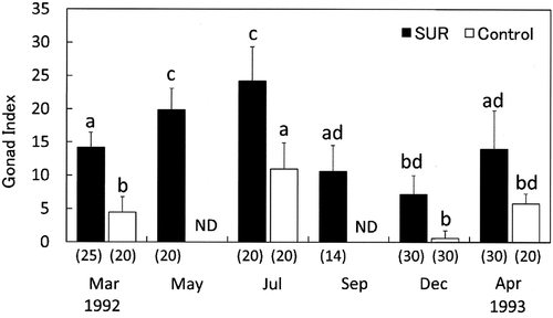
Fig. 9. Effects of sea urchin removal (SUR) on gonadal indices (mean ± SE) of Strongylocentrotus intermedius in the northeastern (NE, Esashi) region from May 1989 to July 1993. Different letters indicate significant differences among months and treatments in a one-way ANOVA with a post hoc comparison using Scheffé’s method. The number of samples is indicated in parentheses. ND, no data.

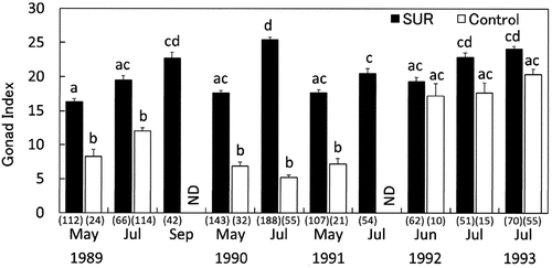
Fig. 10. Relationship between macroalgal biomass and the gonadosomatic index (GSI) of sea urchin in the NE (Esashi) and NW (Rhishiri) regions.

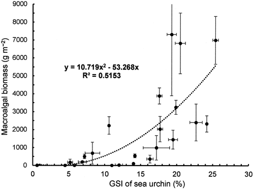
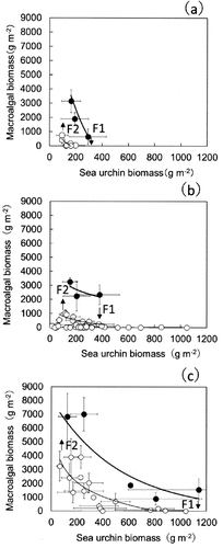
Fig. 11. Relationship between mean sea urchin and macroalgal biomass (mean ± SE) in sea urchin removal experiments. Open circles indicate autumn to winter (September–December) and closed circles indicate spring to summer (March–August). Each season corresponds to the dominant reproductive or vegetative growth season of kelps, which is expressed as bold regression curves. F1 and F2 indicate the highest density of sea urchins with the lowest macroalgal biomass and the lowest density of sea urchins with the highest macroalgal biomass, respectively. These values were determined by using the following equations fitted on the decrease (F1) or increase (F2) of algal biomass by sea urchin removal experiments: (a) Kamiinokuni (SW) F1 ≈ 0.3 kg, y = −4012ln(x) + 2333, r² = 0.94, F2 ≈ 0.1 kg, y = −1014ln(x) + 5345, r² = 0.98, (b) Rishirifuji (NW) F1 ≈ 0.4 kg, y = −2050ln(x) + 14 607, r² = 0.56, F2 ≈ 0.1 kg, y = –427ln(x) + 2771, r² = 0.61, (c) Esashi (NE) F1 ≈ 1.1 kg, y = −2566ln(x) + 19 995, r² = 0.89, F2 ≈ 0.1 kg, y = −2123ln(x) + 14 494, r² = 0.92.