Bent Hansen’s theory of inflation 1951¹

Figures & data

Figure 1. The aggregate perfect competitive goods market under repressed inflation. The price level is set to p₀. The supply curve consists of the aggregate marginal cost curve m. c. up to the quantity Q₁, which is the maximum possible goods production given the available quantity of labour. After that follows a vertical part B₁B₂. The quantitative excess demand in the commodity market equals D₁ - B₁, the ex ante commodity gap equals the area B₁Q₁D₀D₁ and the inflationary gap in the labour market the area B₂Q₁D₀D₁. Excess demand in the aggregate factor market is reflected in how much more goods the firms would like to produce if there was no rationing in the labour market, Q₀ - Q₁. The inflationary gap in the labour market equals the area B₂Q₁Q₀C₁ and unexpected income loss by the firms area B₁B₂C₁. The income loss is equal to the expected profit on production which could not be realised due to shortage of labour.

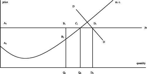
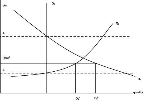
Figure 2. The aggregate goods market under open inflation. Q₁ denotes production given the available labour supply, Q₀ planned supply of goods, D₀ demand for goods, A the level of p/w where the goods market is in equilibrium, B the level of p/w where the labour market is in equilibrium. (p/w)⁰ denotes the quasi-equilibrium value of p/w; here price and wage inflation are equal. In quasi equilibrium the excess demand in the goods market is given by D₀° – Q₁ and the excess demand in the labour market is implicitly given by the distance Q₀° – Q₁ (to measure excess demand in the labour market the distance measured in goods volume has to be transformed to volume of labour via the inverse of the production function).