A protocol for high throughput methods for the expression and purification of inner membrane proteins

Figures & data

Figure 1.  An overall schematic of the expression process using 24, 48 and 96-well systems. (1) Transformation block showing Sections I and II along with the positions of membrane proteins P1–P12 and cell lines C1–C4. (2) 24-well agar plates copying Sections I and II of the transformation block. (3) Block of starter cultures. (4) Two 48-well expression blocks (T₁ and T₂) grown at two different temperatures T1 and T2, respectively. These were set up for each type of media (M1–M4). (5) Representation of analysis blocks M1–M4, showing the final positions of proteins P1–P12, in cell lines C1–C4, grown at temperatures T1 and T2 (labelled T₁ and T₂).

Figure 2.  Sample plates used in the 96-well purification procedure. (a) Standard purification block. This represents the grid system used throughout the 96-well purification procedure. P1–P12 represents 12 different protein samples in columns 1–12. In rows E–H the eight purification detergents D1–D8 are used. (b) Analysis Block 1, used to look for loss of fluorescence during cell lysis, membrane preparation and solubilization. Columns 1–12 contain P1–P12 and rows E–H contain the different samples collected for analysis.

Figure 3.  The 96-well purification procedure. (a) This schematic follows the progress of P1–P12 with 96-well experimental steps being numbered 1–4 and the associated collection blocks denoted 1a–4a, respectively. The analysis plates collected are listed on the right hand side and measurements (Fl, A₂₈₀ and A₃₄₀) taken are listed below them. (b) A table listing the contents of each analysis sample and collection block.

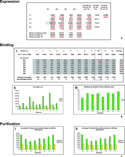
Figure 4.  Examples of typical fluorescence intensity (FI) results (a) Example of FI data collected on a single clone. M1–M4 and C1–C4 denote the different media types and cell lines, respectively. Different growth temperatures, T1 and T2 are shown in black and red, respectively. A box highlights the best condition for the clone and potential calculations of average values across the data are shown. (b) Example of FI results to investigate protein binding. (I) Example data showing the FI values of the starting material (SM) (Block1, Row F) loaded onto the Ni^2 + and the data collected from the flow through (FT) for protein samples P1–P12 in detergents D1–D8 are shown. A box highlights P10 and the greatest (blue) and least (red) binding in the various detergents is highlighted. Potential calculations of average values across the data are shown and the percentage binding calculated. (II) A graph showing the FI value of the SM (green) versus the average FT (yellow) for each protein. (III) A graph showing the binding of P10 in D1–D8. (c) Example of graphs calculated from FI data in elution plates E₁ (green) and E₂ (yellow) (I) Chart showing FI values from P10 in D1–D8. (II) Chart showing average protein elution in D1–D8.