Figures & data
Figure 1. (a) Particle distribution at time (i) 0, (ii) ‘short’, (iii) ‘long’: (b) (i) Particle movement in node plane (ii) interacting particle at separation h. This Figure is reproduced in colour in Molecular Membrane Biology online.
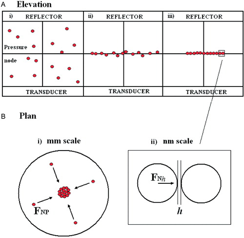
Figure 2. Experimental assembly. The resonator outer diameter is 25 mm. Its main components were a 1.5 MHz disc transducer that was glue-attached to a steel acoustic coupling layer, a sample volume and glass acoustic reflector. The thicknesses of the different layers were selected to give a highly resonant system Citation[24].
![Figure 2. Experimental assembly. The resonator outer diameter is 25 mm. Its main components were a 1.5 MHz disc transducer that was glue-attached to a steel acoustic coupling layer, a sample volume and glass acoustic reflector. The thicknesses of the different layers were selected to give a highly resonant system Citation[24].](/cms/asset/ef800f75-bd54-456f-a833-a58de9d71056/imbc_a_109322_uf0002_b.jpg)
Figure 3. Neural cells suspended in the ultrasound trap: (a) 1 min, and (b) 30 min after initiation of ultrasound. Membrane spreading (grey arrow), blebbing (black arrow) and loss of refractility (dotted arrow) are shown. Scale bar is 25 µm.
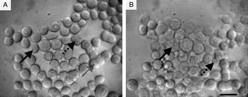
Table I. Decrease in void area and increase in actin filament intensity with time.
Figure 4. Viability assays. (a,b) Staining of dead cells with EthD-1, bright field and fluorescence microscopy respectively at time (t) = 60 min after ultrasound initiation; (c,d) Staining of live cells with Calcein AM (t = 15 min); blebbed cells, but not the blebs, have stained (arrows). (e,f) Dead cells staining with PI. Low refractility cells have been stained (arrows), (t = 60 min); (g,h) Staining of mitochondria of live cells with MiToTracker green FM. Spread cells have stained (arrows), (t = 5 min). Scale bar (a–b) is 250 µm, (c–h) is 20 µm.
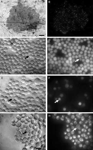
Table II. Responses of cells exposed in situ to different dyes for 1 h in a levitated monolayer.
Figure 5. Development of membrane spreading in an example neural cell doublet: (a) 1 min, (b) 10 min, (c) 20 min, (d) 30 min, (e) 40 min, and (f) 60 min after ultrasound initiation. The ‘outer edge’ separation distance (range 1) and the measured ‘width’ of the tangentially developing contact area (range 2) are shown. Scale bar is 6 µm.
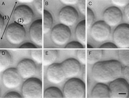
Figure 6. Temporal progression of: (1) the ‘width’ of the developing contact area (dotted line) and (2) the ‘outer edge’ separation distance (continuous line) of selected pairs of spreading cells (error bars indicating the standard error of the mean, n=7). This Figure is reproduced in colour in Molecular Membrane Biology online.
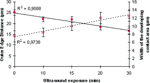
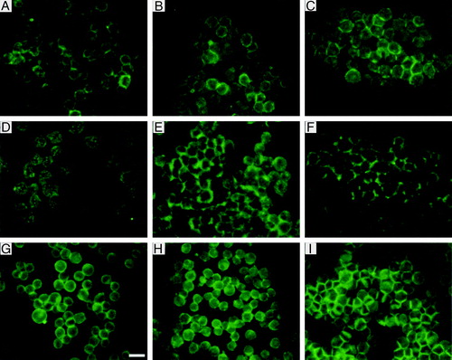
Figure 7. Distribution of NCAM (a–c), N-cadherin (d–f) and actin (g–i) in aggregates isolated from the trap after 1 min (a, d, g), 8 min (b, e, h) and 30 min (c, f, i) of ultrasound initiation. Scale bar is 25 µm. This Figure is reproduced in colour in Molecular Membrane Biology online.