Routing through open spaces – A performance comparison of algorithms

Figures & data

Figure 1. Routing examples using different algorithms (location: Weisenhausplatz, Pforzheim in Germany).

Notes: The gray lines within the open space show the subgraph of the respective algorithm. The black dotted line shows the shortest path from the top-left to the lower-right.

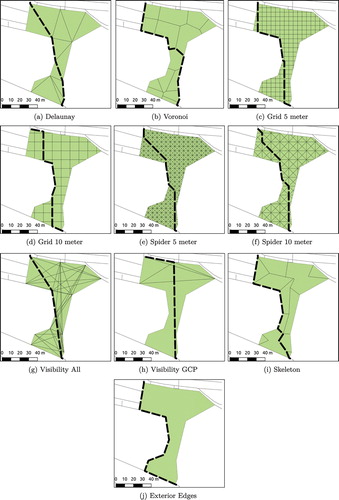
Table 1. Information about study site.

Criterion of comparison	Austria	Baden-Württemberg	Bavaria
Open spaces
Total	3267	5916	5362
Ways	2922	5409	4917
Relations	345	507	445
Processed ways	1889	4654	3372
OSM ways [million]	1.44	1.47	1.90
Created edges [million]	2.46	2.70	3.44
Share	0.23%	0.4%	0.28%

Notes: The top three rows show the total count of open spaces and how many of them are modeled as ways (closed linestrings) and relations (multipolygons). Row four shows the count of the open spaces that were actually processed in the analysis (using the pedestrian profile from GraphHopper). Rows five and six shows the count of ways tagged as “highway” and the count of resulting routing edges without the use of any open space algorithm. The last row shows the share of open spaces on the total count of “highway” ways.

Table 2. Share (%) of failed open space algorithms per test area.

Algorithm	Austria	Baden-Württemberg	Bavaria
Visibility GCP	26	25	31
Visibility All	1	1	1
Delaunay	1	1	1
Voronoi	0	0	0
Grid 5 m	1	1	1
Grid 10 m	4	4	4
Spider 5 m	0	0	0.1
Spider 10 m	0.1	0.1	0.1
Skeleton	1	1	1

Figure 2. Additional edge count and computation duration with usage of CH.

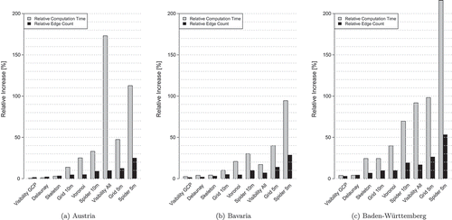
Figure 3. Additional edge count and computation duration without the usage of CH.

Notes: (a) Austria, (b) Bavaria, (c) Baden-Württemberg

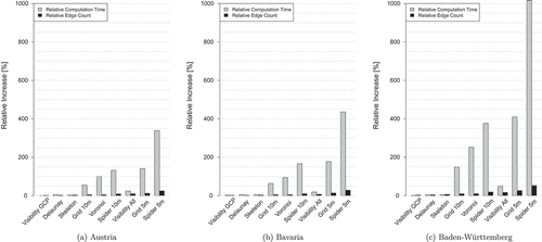
Figure 4. Comparison of graph generation times.

Notes: The percentage value on top of the green bars shows the share of the computation time without CH compared to the computation time with CH. (The computations have been run on a Quad-Core with 2.4 GHz).

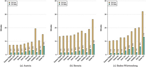
Figure 5. Routing performance.

Notes: (a) Average computation time in milliseconds. (b) Relative increase in computation time compared to Exterior Edges.

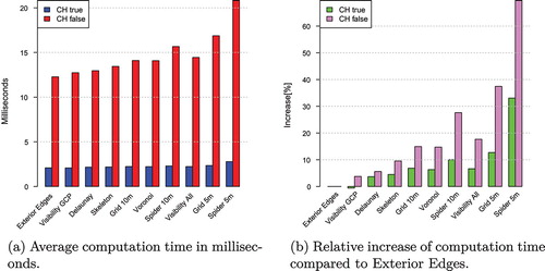
Figure 6. Edge count versus average routing time.

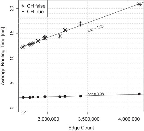
Figure 7. Increased route length compared to Visibility All.

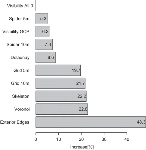
Table 3. Algorithm comparison – usage of CH is considered.