Figures & data
Figure 1. Diagram with the four phases (colored boxes) of the algorithm.
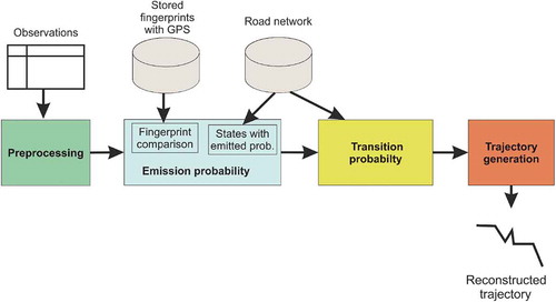
Figure 2. An example of the process of computing the emission probability. It starts with the matching of closest fingerprints using RF (a). Then, it uses the RF distance in meters to select nearby roads for each matched fingerprint (b). Next, the closest points on the roads (dotted circle in green) for each fingerprint (solid circle in grey) are computed (c). Finally, there is a check for close enough points, which are merged together, producing the insertion of blue point in (c), thus obtaining the final set of points (d).
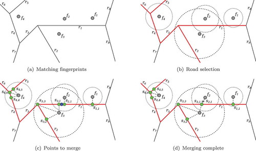
Figure 3. In HMM, the map-matched path is computed by choosing a state and a transition for each observation. States from are represented inside the red box. A possible path is highlighted in bright green.
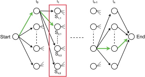
Table 1. An example of the collected fingerprints (GPS data are omitted).
Figure 4. Fingerprint observations collected in the historical centre of Udine, an Italian city. Map Data © OpenStreetMap contributors, CC BY-SA.
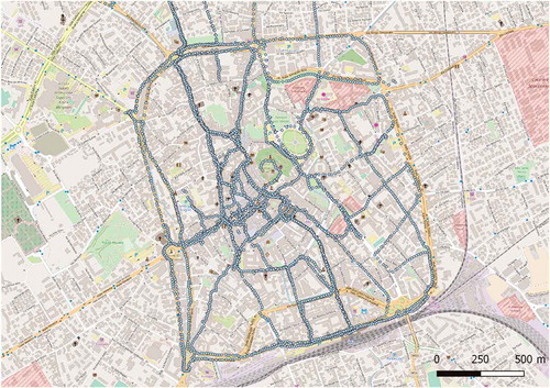
Table 2. Characteristics of the traces used in the evaluation.
Figure 5. The three paths between different points of interests collected in the city of Udine © OpenStreetMap contributors, CC BY-SA.
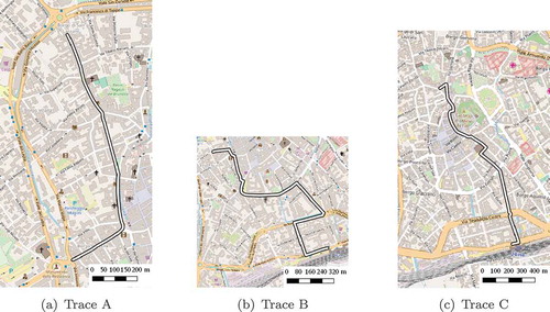
Figure 6. Some intermediate steps of the processing on the trace C, leaving only one observation every 60 seconds. Map Data © OpenStreetMap contributors, CC BY-SA.
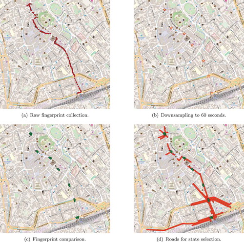
Figure 7. Path A: ground-truth and map-matched trajectory at various samplings. The path goes from the top to the bottom. Map Data © OpenStreetMap contributors, CC BY-SA.
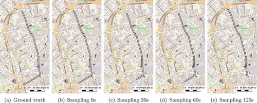
Figure 8. Path B: ground-truth and map-matched trajectory at various sampling rates. The path goes from the top to the bottom. Map Data © OpenStreetMap contributors, CC BY-SA.
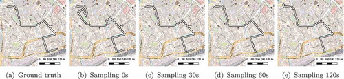
Figure 9. Path C: ground-truth and map-matched trajectory at various samplings. The path goes from the bottom to the top. Map Data © OpenStreetMap contributors, CC BY-SA.
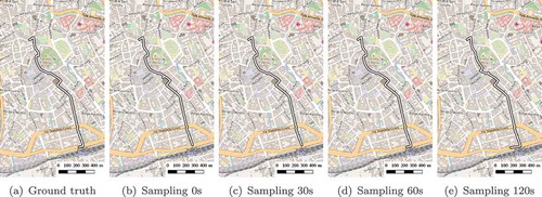
Table 3. Accuracy of the map-matched trajectory using fingerprint observations.
Figure 10. How increasing the sampling time impacts on the recall measures for the different traces.
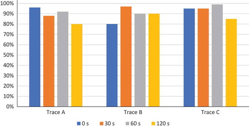
Table 4. Accuracy of the map-matched trajectory with different subsets of fingerprints.
Table 5. Accuracy of the map-matched trajectory using mixed GPS/fingerprint observations.
Figure 11. Recall measures at 120 seconds of sampling for the different traces while taking increasingly larger subsets of the fingerprint map.
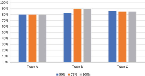
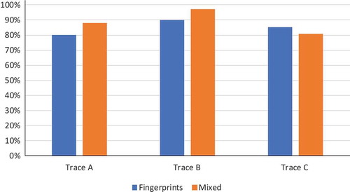
Figure 12. Recall measures at 120 seconds of samplings for mixed sequence (in orange) and fingerprint only sequence (in blue).