Assessing environmental impacts of urban growth using remote sensing

Figures & data

Figure 1. (a) Regions of Wuhan studied for changes in land use. (b) Distribution of Local Government Areas (LGA) in western Sydney. Distances shown in Figures 12 and 13 are measured from the crosses in each figure. (c) Location of Wuhan in China (d) Location of Sydney in Australia.

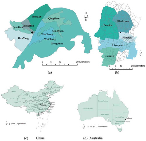
Table 1. Experimental images used for Wuhan and Sydney.

Wuhan			Sydney
Satellite mission	Path / Row	Acquisition Date	Satellite mission	Path / Row	Acquisition Date
Landsat 5	123/039	26^th Sep1987	Landsat 5	090/083	20^th Sep 1988
		12^th Oct 1993			2^nd Sep 1993
		27^th Sep 1999			16^th Sep 1998
		24^th Sep 2004			14^th Sep 2003
		6^th Sep 2009			9^th Sep 2007
Landsat 8		3^rd Oct 2013	Landsat 8		25^th Sep 2013
		30^th Oct 2017			20^th Sep 2017

Figure 2. Landsat data processing flow chart.

Figure 3. Framework of ANN WT (adapted from Mertens et al. (2004)).

Table 2. Accuracy assessment of SRM and pixel-based classification results using available high-resolution images.

		SRM		Pixel-based Classification
		2013	2017	2013	2017
Wuhan	OA	94.6%	92.9%	94.6%	91.6%
	Kappa	0.928	0.905	0.927	0.887
Sydney	OA	82.1%	88.3%	80.4%	87.5%
	Kappa	0.762	0.844	0.739	0.834

Figure 4. Comparisons of SRM results in Wuhan from year 1987 (a) to 2017 (b) and in Sydney from 1988 (c) left to 2017 (d).

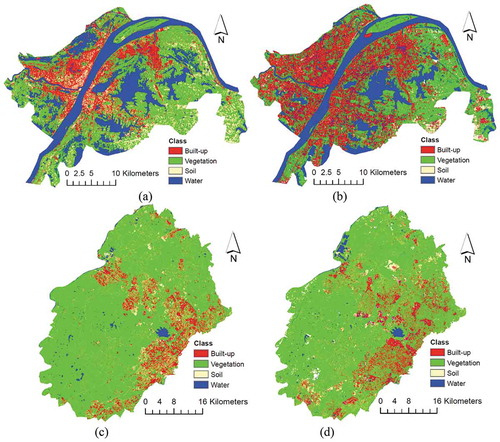
Figure 5. Results at fine-scale showing the comparison between pixel-based classification (using MESMA) and SRM. The left column shows results for Wuhan (the year 2017) and the right for western Sydney (the year 2013). (a) and (b) are reference high-resolution images for Wuhan and Sydney, respectively (c) and (d) pixel-based classification results for Wuhan and Sydney, respectively. (e) and (f) SRM results for Wuhan and Sydney, respectively. Built-up, vegetation, soil and water are represented by red, green, yellow and blue color, respectively.

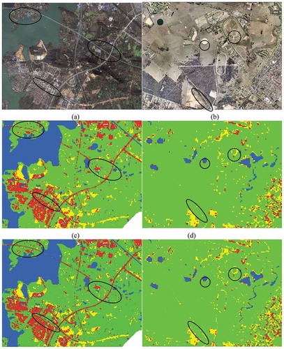
Figure 6. Objects mean sizes (m²) for four classes of buildings, soil, vegetation and water in Wuhan.

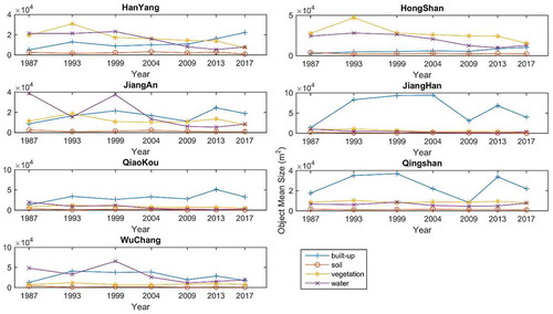
Figure 7. Object mean sizes (m²) for four classes in western Sydney. Class built-up, soil and water are indicated in the left axis and vegetation in the right axis.

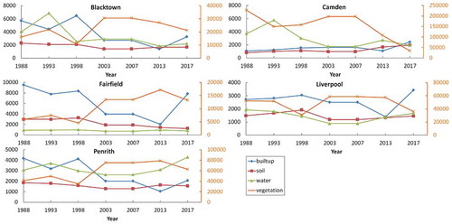
Figure 8. The number of objects in Wuhan for four classes of buildings, soil, vegetation and water.

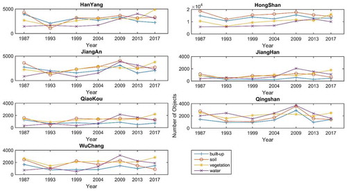
Figure 9. The number of objects in western Sydney for four classes of buildings, soil, vegetation and water.

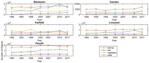
Figure 10. Object density (no./km²) in Wuhan for four classes of buildings, soil, vegetation and water.

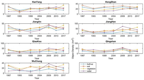
Figure 11. Object densities (no./km²) in western Sydney for four classes of buildings, soil, vegetation and water.

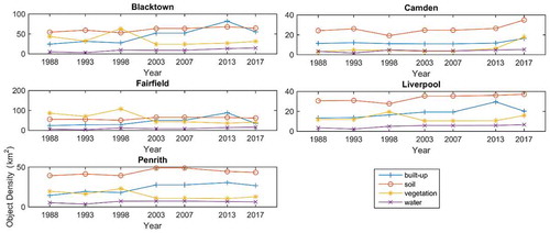
Figure 12. Growth and loss in vegetation objects in terms of distance (a) and orientation (b) from the center of Wuhan (km²).color

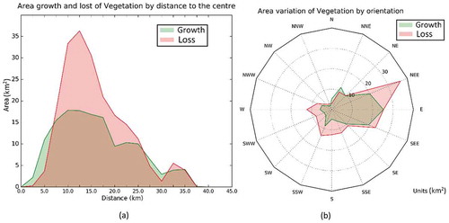
Figure 13. Growth and loss in vegetation objects in terms of distance (a) and orientation (b) from the center of western Sydney.

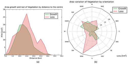
Figure 14. Areal rates (%) of change of vegetation (a) and annual change (km²/year) (b) in QiaoKou region and JiangHan region in Wuhan from 1987–2017.

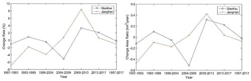
Table 3. Values of ESV for classifications extracted in Wuhan and Sydney.

Ecosystem services	Equivalent classifications in this paper	2007$/ha/yr
Grassland/Rangeland/Cropland	Vegetation and soil	4867
Lakes/rivers	Water	12512
Urban areas	Buildings	6661

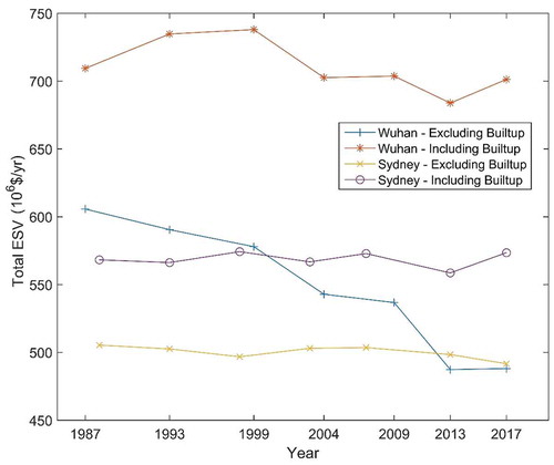
Figure 15. ESVs for Wuhan and Sydney derived from ESVs from (i) vegetation + soil + water, and (ii) vegetation + soil + water + urban, according to accompanying legend.

Mertens, K. C., P. C. Lieven, T. W. Verbeke, and R. R. De Wulf. 2004. “Sub-pixel Mapping and Sub-pixel Sharpening Using Neural Network Predicted Wavelet Coefficients.” Remote Sensing of Environment 91 (2): 225–236. doi:10.1016/j.rse.2004.03.003.

 Web of Science ®Google Scholar