Figures & data
Figure 1. Traffic volume assessment process.
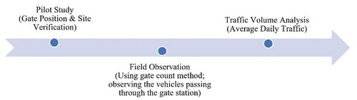
Figure 2. Neighborhood with an upper middle-class background.
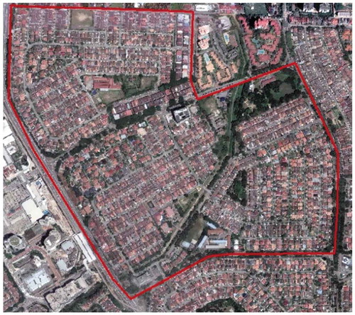
Figure 3. Example of observer line and observation tabulation form (Al-Sayed et al. Citation2014). (a) Gate position and observer line. (b)Observation tabulation form.
Figure 4. Process of generating 3D modeling using GIS and Rhinoceros 3D. (a) #Points cloud generated from the GIS database in Rhinoceros 3D. (b) #Final 3D#model of layout executed from the points cloud.
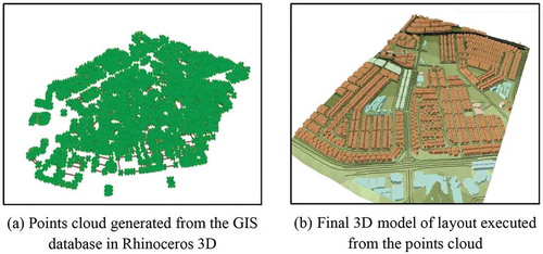
Figure 5. Measuring direct visibility using isovist model builder in Grasshopper. (a) Isovist model builder in Grasshopper for direct visibility. (b) Measuring visibility on the layout.
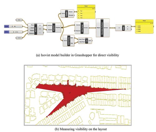
Figure 6. Areas with higher concentration of traffic.
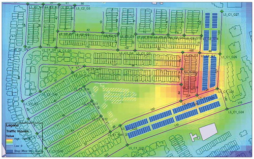
Table 1. Degree of visibility of each parameter for residential land use.
Table 2. Degree of visibility of each parameter for commercial land use.
Figure 7. Concentration simulation of integration.
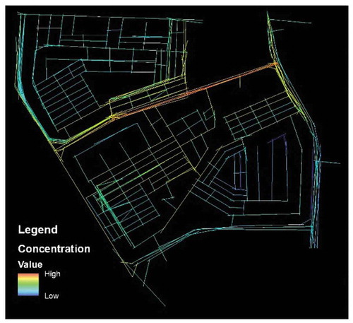
Figure 8. Concentration simulation of connectivity.
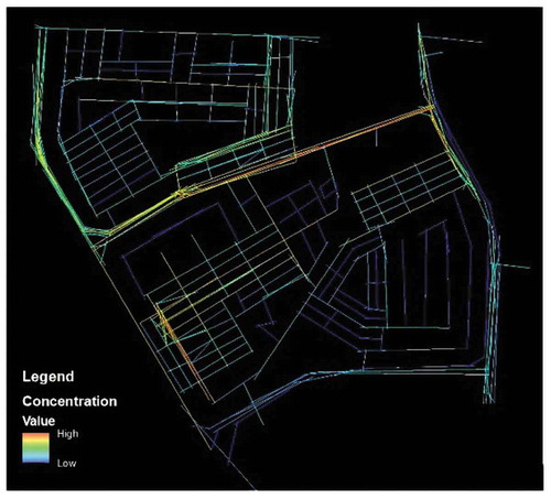
Figure 9. Concentration simulation of choice.
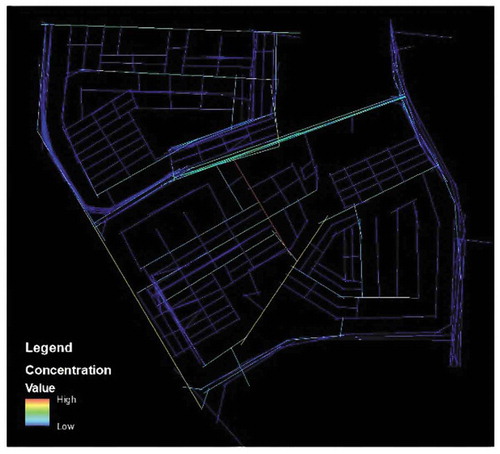
Figure 10. Concentration simulation of direct visibility.
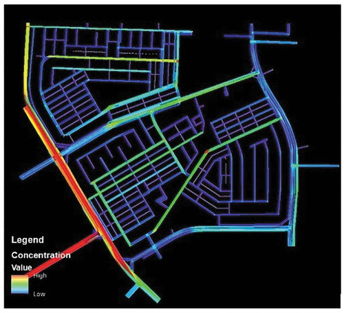
Figure 11. Multiple regression analysis between space parameters and average daily traffic volume. (a) Degree of choice. (b) Degree of integration. (c) Degree of connectivity. (d) Degree of visibility (3D). (e) Degree of visibility (2D).