
Figures & data
Figure 1. System integration: In this MMS, GNSS/INS, 3D LiDAR scanner and panorama camera are mounted on the frame, and the frame’s cabinet also includes firmware such as time synchronizer and GNSS receiver
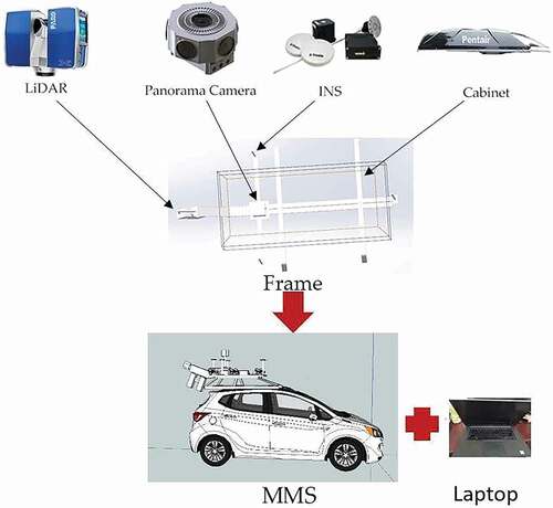
Table 1. INS parameters (Applanix Citation2002)
Table 2. 3D LiDAR scanner parameters (Faro Citation2014)
Figure 2. Technical Roadmap: It is mainly divided into four steps: Firstly, obtaining the initial calibration value; Secondly, establishing the calibration field; Thirdly, calculating the correction; Finally, evaluating the accuracy
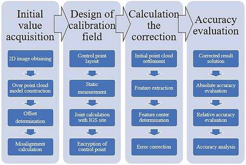
Table 3. The technical parameters of Leica TS30 (Leica Citation2009)
Figure 3. The layout of reflectors around MMS: A total of 27 reflectors are pasted on the MMS, among them, the red box is the verification point, and the yellow box is the control point
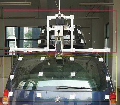
Figure 4. 2D image and point cloud model of MMS: (a) The 2D image of MMS is taken by digital camera, which can be used to generate refined 3D point clouds. (b) The point cloud model of MMS generated by 2D image, that could well reflect the spatial relationship of each sensor in MMS
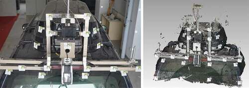
Table 4. The coordinates of verification points
Figure 5. Center of Panorama camera: a) Side view of panorama camera point cloud with the center of the cross as the center of panorama camera; b) Top view of panorama camera point cloud with the center of “X” being the center of panorama camera
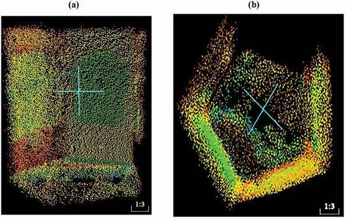
Figure 6. Joint Settlement Based on IGS Stations: point distribution map, in this paper, six IGS control points are selected for adjustment; Results of adjustment Among them, points g03-g06 are the primary control points selected in this paper. From the Table, it can be seen that the adjustment errors are all less than 0.005 m
Figure 7. Schematic diagram of target ball: 1) reflector 2) horizontal platform 3) horizontal bubble 4) spherical surface 5) support rod 6) base
Figure 8. Distribution of feature points: A total of 17 special target balls were set up as marking points and evenly distributed on both sides of the road in the calibration field. (As the red circle)
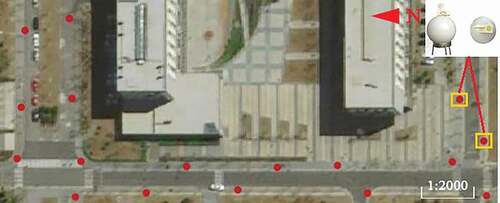
Figure 9. Feature points of building facades: The feature points such as window corners (the red box) and wall corners (the yellow box) were selected in the facade of a building in the calibration site
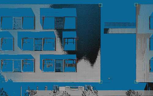
Figure 10. Flow chart of calibration: An error calibration model is established by combining the coordinates of control points measured by a high-precision total station and MMS, so as to calculate the offset and the misalignment error correction
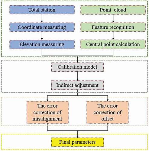
Figure 11. The flow of the experiment: 1) planning a route: The first step in the data collection experiment. After setting the driving route, we can ensure that we can collect all kinds of point cloud data we need. 2) laying a base station: The role of the base station is to receive satellite signals and transmit them to the GNSS system of the MMS to ensure that the position information of the MMS can be updated in real time during data acquisition. 3) acquiring data: After completing the preparation for the experiment, we can begin to collect data. In the process of collecting data, we should as far as possible to avoid areas with weak satellite signals and drive at a constant speed. 4) preprocessing the data: This step includes coordinate transformation and registration of point cloud data, in this paper, we completed it through our own MMS data processing software
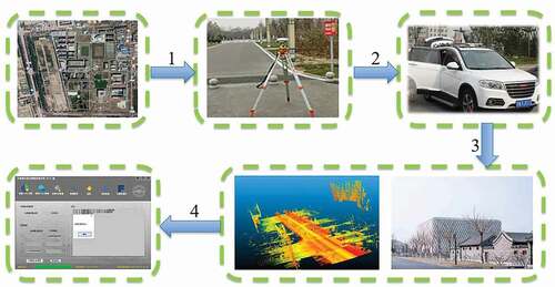
Figure 12. Location Map of Base Stations and Control Points: In the Figure, the red line is part of the driving route, the yellow circle is the GNSS base station (WGS84), and the yellow Pentagram is the control point
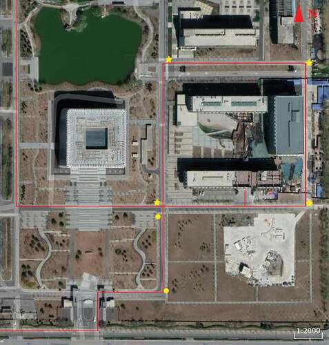
Figure 13. The point clouds collected by the MMS
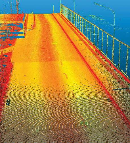
Figure 14. Driving track: Driving trajectory is the basis of data fusion calculation. Combining trajectory with planned driving route analysis can quickly find the point cloud area where the feature points are located (WGS84)
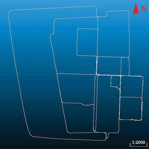
Figure 15. Point cloud solution software: The self-developed MMS processing software using C# language. Through this software, the scanner can be operated during the working process of the MMS, and the data can be pre-processed such as registration and coordinate transformation after data acquisition is completed
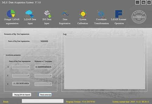
Figure 16. Layout of target balls: In the area that can be scanned by the MMS, a special target ball is arranged in a place with a wide field of vision and can be viewed back and forth, so that the measurement by the total station is more convenient and the measurement result is more accurate
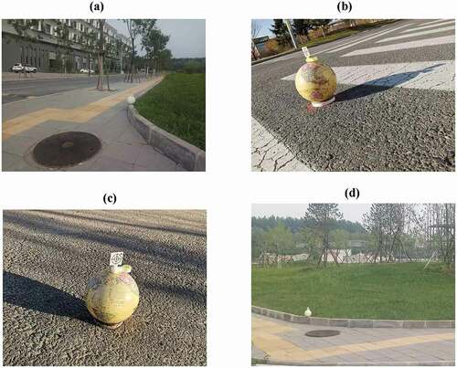
Table 5. Absolute error of MMS before calibration
Table 6. Absolute error of MMS before calibration
Table 7. Absolute error of MMS after calibration
Figure 17. Comparison diagram of a building’s point cloud before and after calibration (a) Front view of a building before and after calibration; (b) Top view of a building before and after calibration (In the above figures, the green point cloud is the point cloud data before calibration, and the white point cloud is the point cloud data after calibration)
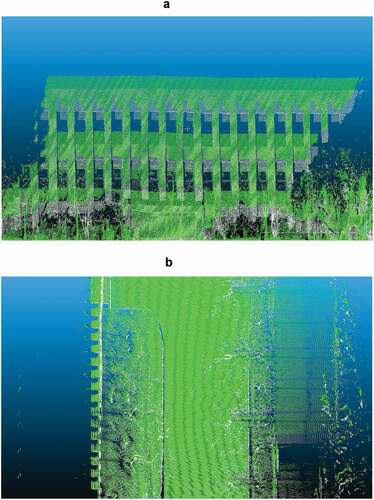
Figure 18. Partial point cloud data on and from stations: (a) guard room data obtained by TLS; (b) windowsill data obtained by TLS; (c) guard room data obtained by MMS; (d) windowsill data obtained by MMS
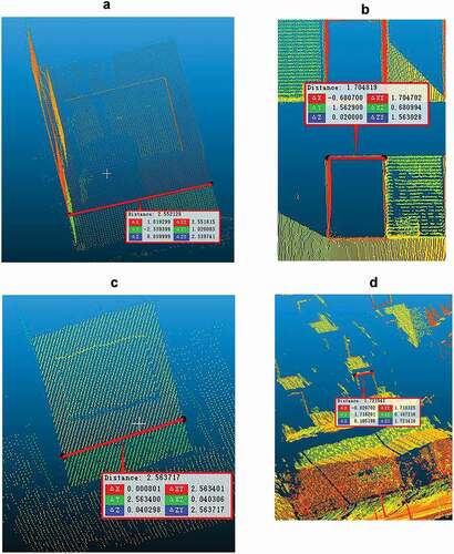
Table 8. Data of TLS control group
Figure 19. Outdoor tape measurement: (a) the street tree diameter measurement site; (b) the stone pier height measurement site; (c) the street lamp pole diameter measurement site
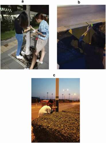
Table 9. Data of tape control group
Figure 20. Chromatogram of point cloud TLS and MMS of a building: In this figure, the colored part is the overlapping part of the TLS point cloud data model and the MMS point cloud data, and the gray part did not participate in the comparison due to the lack of point cloud data
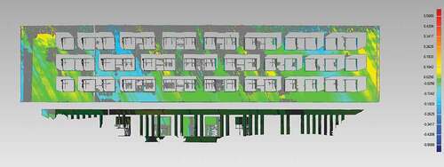
Figure 21. Windowsill point cloud 3D model: In the Figure, yellow and green are the 3D models encapsulated by the point cloud data of the TLS, and red points are the point cloud data of the MMS
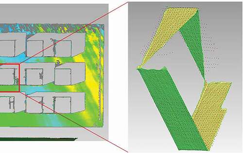
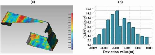
Figure 22. 3D analysis results of windowsill model: (a) 3D analysis chromatogram, tolerance is −0.01 m – 0.01 m, turquoise is more observed from the Figure, indicating that the overall deviation is smaller (b) overall deviation distribution diagram, deviation is approximately positive distribution, and most deviation is within 0.005 m
Data availability statement
The data that support the findings of this study are available from the corresponding author, [Jianghong Zhao], upon reasonable request.