i4sea: a big data platform for sea area monitoring and analysis of fishing vessels activity

Figures & data

Figure 1. Overall architecture.

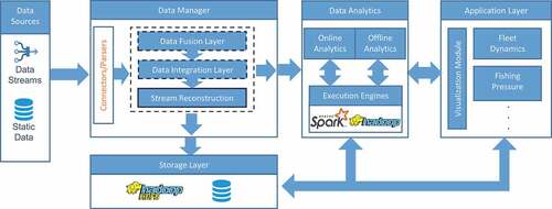
Figure 2. The (a) VMS trace, (b) AIS trace and (c) Fused trace of a specific fishing vessel.

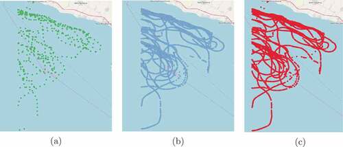
Figure 3. Overall architecture.

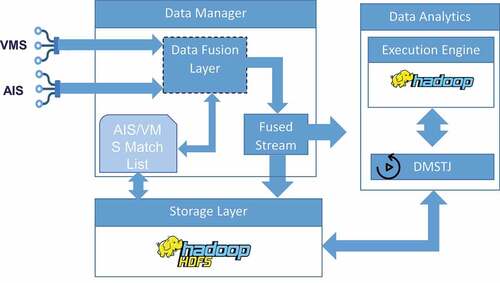
Figure 4. Two raw trajectories (in blue) and their corresponding synopses (in red).

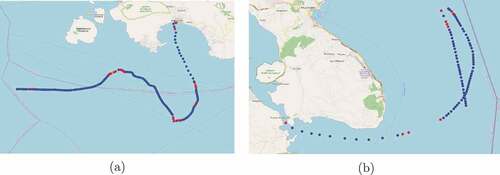
Figure 5. Overall architecture.

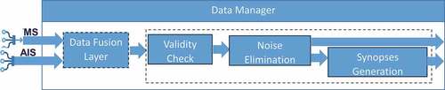
Figure 6. Mobility data enrichment streaming pipeline.

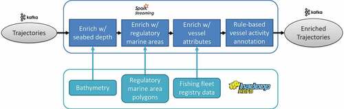
Figure 7. A pair of maximally “matching” subtrajectories $(r_{4,8},s_{3,7})$.

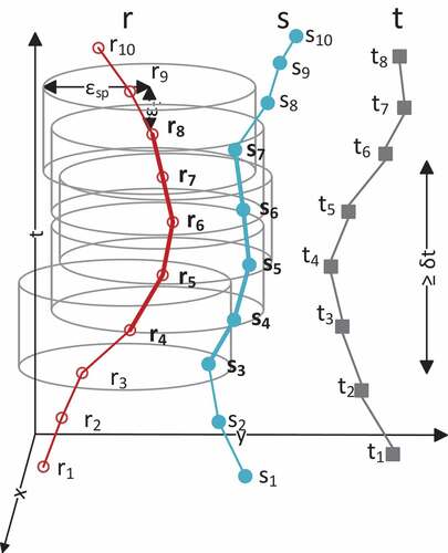
Figure 8. Clustering example of six trajectories moving in an intersection.

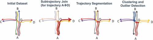
Figure 9. Data points are mapped to and grouped by cells, yielding a dataset of cells with a specific value.

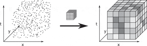
Figure 10. Data locality in Hotspot Analysis. A worker is processing the partition with white cells. Gray cells denote exterior cells of neighboring partitions that are transmitted to the worker, so that the whole neighborhood of each white cell is made locally available to the worker.

Figure 11. Network architecture for the proposed LSTM model, with one LSTM cell and two fully connected layers. The dark blue boxes indicate layers in the network, while the light blue ones indicate the input-output information.

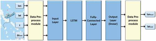
Figure 12. Activity prediction pipeline.

Figure 13. Application prototype for online analytics results monitoring.

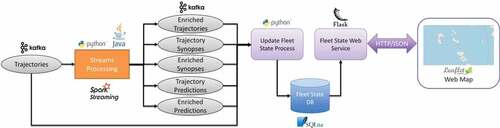
Figure 14. Fishing vessel activity view of the online analytics results monitoring application prototype. A fishing vessel is depicted as either mooring, steaming, or fishing.

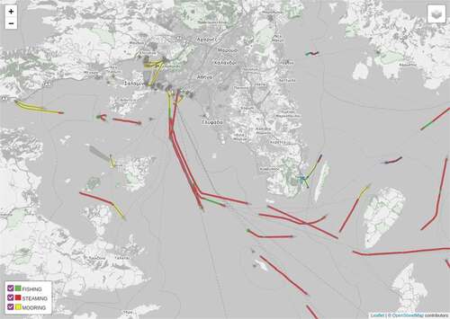
Table 1. AIS/VMS fusion confusion matrix with accuracy and precision

	Discovered				Accuracy	Precision
Actual		True	False	Total	0.833493	0.846154
	Positive	44	166	210
	Negative	8	827	835
	Total	52	993	1045

Figure 15. Examples of discovered matches between VMS (red) and AIS (green).

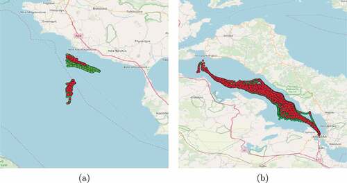
Table 2. Compression rate of Synopses Generator

Number of Positions	Critical Points	Compression Rate
101281869	11778948	88.37%

Figure 16. Performance of the Synopses Generator in terms of latency.

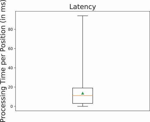
Table 3. Experimental evaluation of online mobility data enrichment in Apache Spark Streaming. Noise-free AIS traces vs AIS Synopses processed using trigger interval option set to 1, 2, 4 and 8 minutes

	Median Latency (in msec)
Trigger Interval	Noise-Free Raw Data	Synopses
1	31.54	2.87
2	60.33	5.35
4	115.67	10.32
8	226.21	20.67

Figure 17. Comparison between DSC, S²T-Clustering and TraClus in terms of the RMSE metric.

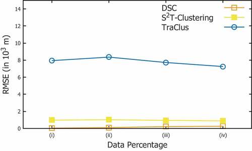
Figure 18. Fishing Pressure Hotspot Analysis of trawler AIS data. The data spans one month from 1 January 2018 to 31 January 2018 and is temporally grouped by the whole temporal range. The figure displays (a) the overview and (b) a detail of the analysis result.

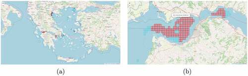
Figure 19. Fishing Pressure Hotspot Analysis of purse seiner AIS and VMS data at depths greater than 50 m. The data spans eight months from 1 January 2018 to 31 August 2018 and is temporally grouped by 15-day timespans. The figure displays (a) the overview and (b) a detail of the analysis result.

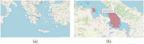
Figure 20. Fishing Pressure Hotspot Analysis of trawler AIS complete data in contrast to AIS synopses data. The data spans three months from 1 January 2018 to 31 March 2018 and is temporally grouped by 15-day timespans. The figure displays two details of the analysis result for the AIS complete data in (a) and (c) and the corresponding details of the analysis result for the AIS synopses data in (b) and (d). AIS synopses data, although much sparser than AIS complete data, seems to perform well enough in this case, successfully identifying the vast majority of hotspots.

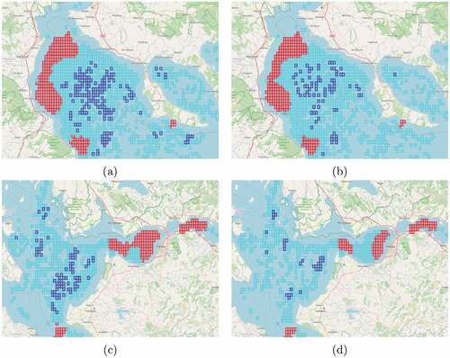
Figure 21. Toward the exploitation of EvolvingClusters in Maritime Domain (left: MCS; right: MC). Discovering anchorages and (potential) fishing areas.

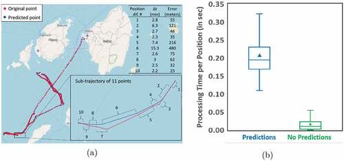
Figure 22. (a) Original locations vs Predicted locations for a fishing vessel and (b) Performance of the FLP tool in terms of latency.

Data availability statement

The AIS and VMS datasets used in our experimental study cannot be made publicly available due to national legislative constraints. However, a subset of the AIS dataset which was collected by our AIS antenna can be found at https://doi.org/10.5281/zenodo.4498410.