Evaluation of wave retrieval for Chinese Gaofen-3 synthetic aperture radar

Figures & data

Figure 1. (a) Calibrated vertical-vertical (VV) polarization quick-look image of Gaofen-3 (GF-3) Synthetic Aperture Radar (SAR) image captured on 21 January 2020 at 10:11 UTC in the coastal waters of the East China Sea. (b) Information on GF-3 SAR images collected from January to July 2020, in which the rectangles represent the spatial coverage.

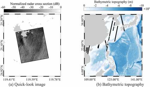
Figure 2. Simulated region for the simulating waves nearshore (SWAN) model and the unstructured grid.

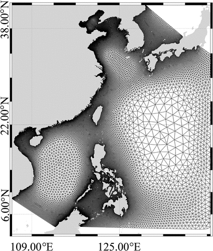
Figure 3. (a) Wind map from European Center for Medium-Range Weather Forecasts (ECMWF) reanalysis ERA-5 data on 21 January 2020 at 10:00 UTC. (b) Current speed map from the hybrid coordinate ocean model (HYCOM) on 21 January 2020 at 09:00 UTC. (c) Sea surface elevation from HYCOM on 21 January 2020 at 09:00 UTC. (d) Sea surface temperature from HYCOM on 21 January 2020 at 09:00 UTC. Note that the black rectangle represents the spatial coverage of the image in Figure 1(a).

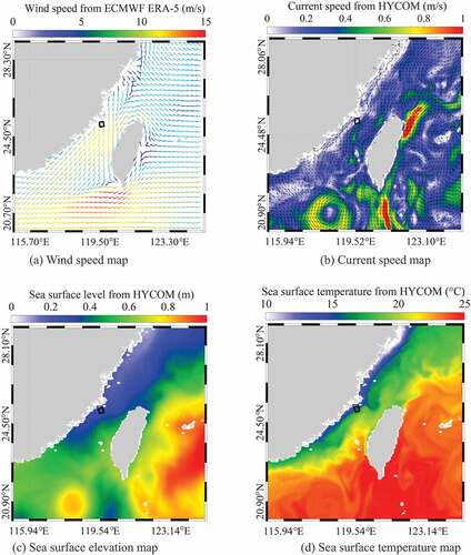
Figure 4. (a) Significant wave height (SWH) map for 17:00 UTC on 19 January 2020. The satellite footprint is shown as colored boxes overlaid on the SWAN-simulated SWH field. (b) Corresponding ECMWF SWH map.

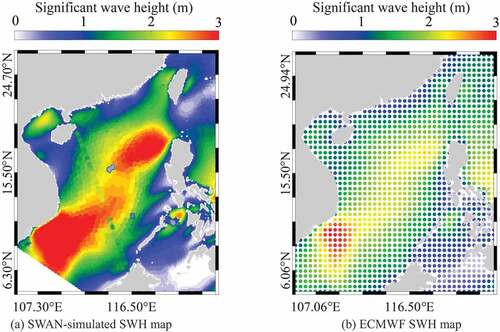
Figure 5. SWAN-simulated SWH compared with the measurements from the Jason-3 altimeter 3 for the period from January to July 2020.

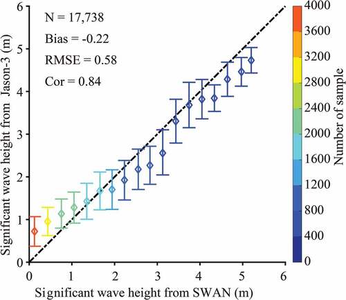
Figure 6. One-dimensional spectrum using the Elfouhaily (E-spectrum) and JONSWAP wave spectrum at a wind speed of 8 m/s.

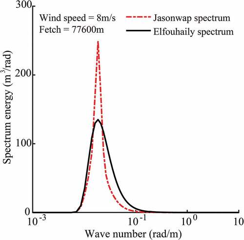
Figure 7. Flowchart of the wave retrieval scheme used in this study.

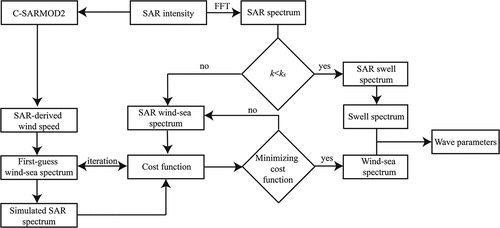
Figure 8. SAR-derived wind map using C-SARMOD2 from the GF-3 SAR image taken on 21 January 2020 at 10:11 UTC.

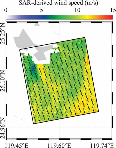
Figure 9. Validation of SAR-derived wind speeds with ECMWF reanalysis (ERA-5) winds for the period from January to July 2020. The color represents the data density in 0.2 m/s bins.

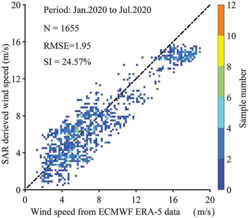
Figure 10. (a) Example of the subscene in Figure 1(a) covering the SWAN grids. (b) Corresponding SAR two-dimensional spectrum. (c) SAR-derived and SWAN-simulated one-dimensional spectrum.

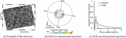
Figure 11. (a) Comparison between SWAN-simulated SWH and SAR retrieval SWH using the parameterized first-guess spectrum method (PFSM). (b) Comparison between SWAN-simulated SWH and SAR retrieval SWH using the proposed algorithm.

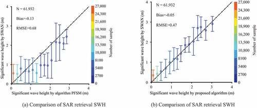
Figure 12. The high frequency radar part results. (a) Comparison between SWAN-simulated SWH and SAR retrieval SWH using the parameterized first-guess spectrum method (PFSM). (b) Comparison between SWAN-simulated SWH and SAR retrieval SWH using the proposed algorithm.

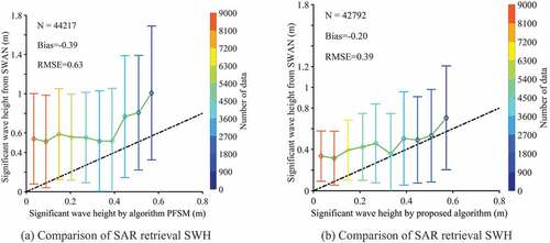
Figure 13. Bias (SAR-derived SWH using the proposed algorithm minus SWAN-simulated SWH) is contrasted with (a) SAR-derived wind speed, (b) sea surface current speed from HYCOM model, (c) sea surface elevation from HYCOM model, and (d) sea surface temperature from HYCOM model.

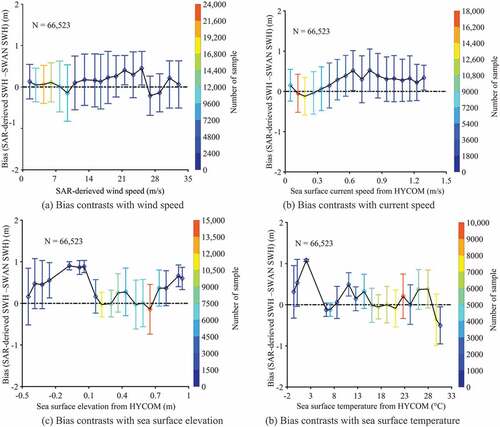
Table A1. Settings for the Simulating WAves Nearshore (SWAN) (41.31) model

Forcing field	ECMWF ERA-5 wind with a spatial resolution of 0.5° and a time interval of 1 h; sea surface current speed and sea water elevation from HYCOM with a spatial resolution of 0.08° and a time interval of 3 h.
Frequency bins	Logarithmic between 0.01 and 1 at an interval of Δf/f = 0.0903
Resolution	A 30-min temporal resolution
Bulk formula	High wind speed bulk formula in Ou et al. (2002) for white-capping
Other settings	Wave-interactions (QUADrupl), triad wave-wave interactions (TRIad), and bottom friction (FRICtion)

Ou, S.H., J.M. Liau, T.W. Hsu, and S.Y. Tzang. 2002. “Simulating Typhoon Waves by SWAN Wave Model in Coastal Waters of Taiwan.” Ocean Engineering 29 (8): 947–971. doi:10.1016/S0029-8018(01)00049-X.

 Web of Science ®Google Scholar

Data availability statement

The data that support the findings of this study are available from the corresponding author upon reasonable request.