Artificial intelligence and remote sensing for spatial prediction of daily air temperature: case study of Souss watershed of Morocco

Figures & data

Figure 1. Map of the Souss watershed showing the selected weather stations.

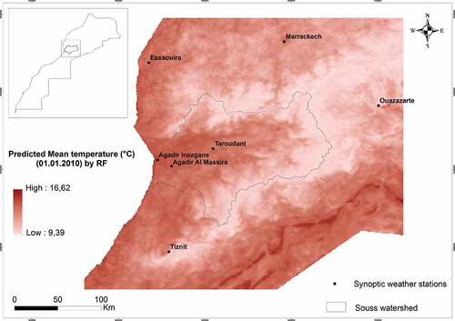
Figure 2. MODIS predictor variables for 01/01/2019: Terra Band 32 Emissivity (TE32, unitless, with a 0.002 scale factor), Terra Nighttime Land Surface Temperature (TLSTN, in kelvin with a scale factor of 0.02), Terra local time of night observation (TNVT, in hours with a scale factor of 0.1), Aqua Band 31 Emissivity (AE31, unitless, with a scale factor of 0.002), Aqua Daytime Land Surface Temperature (ALSTD, in kelvin with a scale factor of 0.02) and Aqua Nighttime Land Surface Temperature (ALSTN, in kelvin with a scale factor of 0.02).

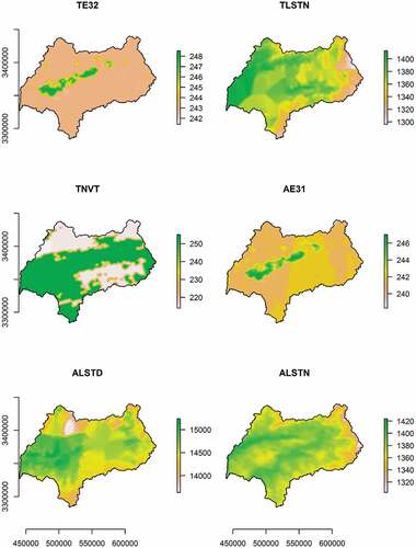
Figure 3. Auxiliary predictor variables used in the study (elevation in meters, slope in degrees).

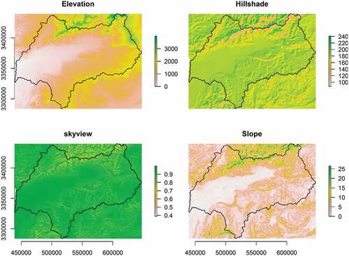
Table 1. Statistical and Machine learning methods used for Tair prediction

Method	Description
Linear Regression	Linear regression is a statistical approach that is used to find a linear relationship between the target and one or more predictors. From the target variable (Y), the model aims at making a prediction thanks to the predictor variable (X). Y is usually quantitative, while X can be quantitative or qualitative. The objective is to find a prediction function or a cost function that describes the relationship between X and Y.
Partial Least Squares (PLS)	Based on integration and development of multiple linear regression, canonical correlation analysis, and principal component analysis. Strength lies on its ability to analyze data with strongly collinear, noisy, and numerous (Eriksson et al. 2001).
K-Nearest Neighbors (KNN)	Nonparametric, lazy learning algorithm suitable when there is little or no prior knowledge of the data distribution. Instance-based learning approach where a class label is assigned to a new instance based on the closest correctly classified neighboring instances. Hamming and Euclidean distances are used for discrete and continuous variables, respectively. KNN is based on distance for classification. Thus, if the features represent different physical units or occur at very different scales, normalizing the training data can greatly improve its accuracy. Moreover, it takes all cases contributing to the dataset and ranks the new cases based on their similarity indices. Cases are ranked by voting for neighboring classes, with the optimal case having the highest similarity indices (Wu et al. 2008).
Cubist	Rule-based regression technique that was developed based on a combination of the ideas of Quinlan (1992, 1993). Popular and widely used regression and classification method because due to being ported into R. Has been used in Tair estimation research and showed very good results. Meyer et al. (2016) in mapping daily Tair in Antarctica and Zhang et al. (2006) in estimating daily Tair over the Tibetan plateau in China.
Extreme Gradient Boost (XGB)	Based on aggregation of decision trees. During each iteration, new tree is trained based on the error of the preceding tree Can be used for both classification and regression problems High execution speed out of core computation (Chen and Guestrin 2016) While characterized by generally accurate estimates, the gradient boosting approach can be prone to overfitting. XGB overcomes this limitation by adding a regularization term in the objective function.
Random Forest (RF)	RF, which were proposed by Breiman (2001). Nonparametric, tree-based ensemble technique; Easy to interpret Independent decision trees; developed from bagged set of trees (tree-bagging) In the case of bagging, a number of decision trees are created, each tree being created from a different bootstrap sample of the training dataset. This bootstrap sample refers to a sample of the training dataset where an example may appear more than once in the sample. This is called ”sampling with replacement”. RF operates on multiple decision trees randomly trained on different subsets Final predicted values are produced by the aggregation of the results of all the individual trees that make up the forest (Xu, Knudby, and Ho 2014)

Table 2. Selected variables for PLS, RF, and XGB using forward feature selection

All variables	Models	Selected variables
ACDC (Aqua day clear-sky coverage), ACNC (Aqua night clear-sky coverage), ADVA (Aqua day view angle), ADVT (Aqua day view time), AE31 (Aqua Band 31 Emissivity),AE32 Aqua Band 32 Emissivity, ALSTD (Aqua day land surface temperature), ALSTN (Aqua night land surface temperature), ANVA (Aqua night view angle), ANVT (Aqua night view time),TCDC (Terra day clear-sky coverage),TCNC (Terra night clear-sky coverage), TDVA (Terra day view angle), TDVT (Terra day view time),TE31 (Terra Band 31 Emissivity), TE32 (Terra Band 32 Emissivity),TLSTD (Terra day land surface temperature), TLSTN (Terra night land surface temperature), TNVA (Terra night view angle), TNVT(Terra night view time), Elevation (DEM), Hillshade (HSD), Sky-view, Slope	PLS	ALSTN, TLSTN, HSD, ADVT, ALSTD, ANVA, TLSTD, TCNC, ADVA, TNVA, TNVT
	RF	TE32, TLSTN, ALSTN, ALSTD, TNVT, AE31
	XGB	TE32, TLSTN, ALSTN, AE32, ADVT, DEM, TCNC, TDVT, TLSTD

Figure 4. Relative variable importance for the algorithms used.

Figure 5. Agreement between measured air temperature and predicted air temperature using RF model as modeling tool. Models were first trained using the full set of predictor variables (ALL) and second using only selected variables as predictors that were revealed during forward feature selection (FS). Two different validation strategies were used: Comparison to a 70% random subset of the total dataset (RS), as well as Leave-One -Out Cross-Validation (LCV).

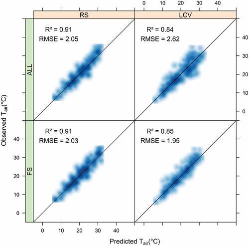
Figure 6. Correlation between measured and predicted air temperature based on KNN, PLS, XGB, XGBD, LM1, LM2, CUBIST, and RF models.

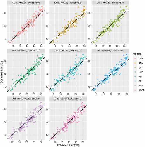
Figure 7. Distribution of residuals versus fitted air temperature based on KNN, PLS, XGB, XGBD, LM1, LM2, CUBIST, and RF models.

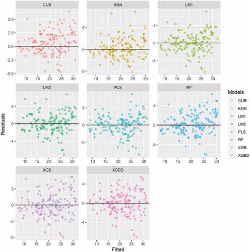
Figure 8. Time series for weather stations: Agadir Al Massira, Essaouira, Marrakech, and Ouarzazate weather stations for 2010–2019 period.

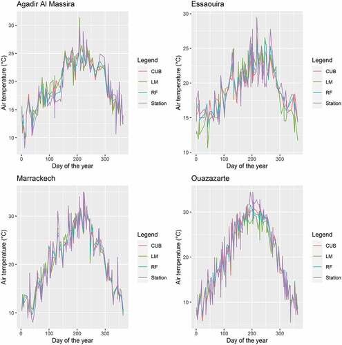
Figure 9. Station dependent errors: (a) RMSE for RF model, (b) Rsq for RF model, (c) RMSE for CUBIST model, (d) Rsq for CUBIST model, (e) RMSE for KNN model, (f) Rsq for KNN model, (g) RMSE for LM1, (h) Rsq for LM1, (i) RMSE for LM2, (j) Rsq for LM2, (k) RMSE for PLS model, (l) Rsq for PLS model, (m) RMSE for XGB model, (n) Rsq for XGB model, (o) RMSE for XGBD model, (p) Rsq for XGBD model. (For the stations: 1 = Agadir Al Massira, 2 = Essaouira, 3 = Marrackech and 4 = Ouarzazate.).

Figure 10. Monthly aggregates of air temperature for 2010 as predicted by the RF model.

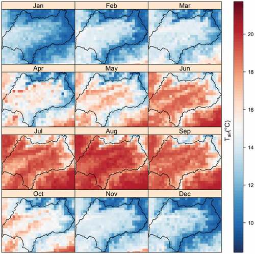
Figure 11. Daily air temperature for 2010 as predicted by the RF model.

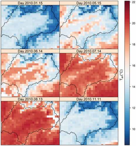
Figure 12. Monthly aggregates of air temperature for 2015 as predicted by the RF model.

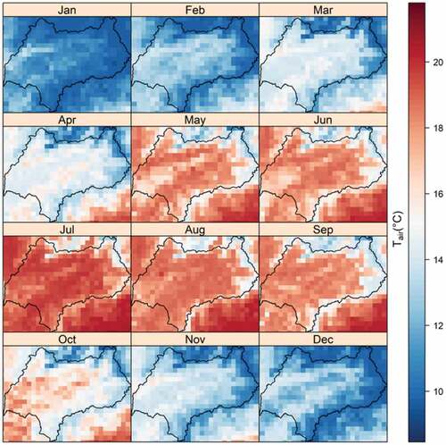
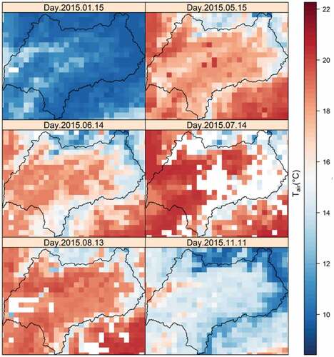
Figure 13. Daily air temperature for 2015 as predicted by the RF model.

Eriksson, L., E. Johansson, N. Kettaneh-Wold, and S. Wold. 2001. Multi- and Megavariate Data Analysis: Principles and Applications. Sweden: Umetrics AB.

 Google Scholar

Wu, X., V. Kumar, J.R. Quinlan, J. Ghosh, Q. Yang, H. Motoda, G.J. McLachlan, A. Ng, B. Liu, and S.Y. Philip. 2008. “Top 10 Algorithms in Data Mining.” Knowledge and Information Systems 14: 1–37. doi:10.1007/s10115-007-0114-2.

 Web of Science ®Google Scholar

Quinlan, J.R., 1992. “Learning with Continuous Classes.” In Proceedings of the 5th Australian Joint Conference on Artificial Intelligence, 343–348. Hobart, Tasmania, November 16–18.

 Google Scholar

Quinlan, J.R., 1993. “Combining Instance-based and Model-based Learning”. In Proceedings of the Tenth International Conference on Machine Learning, 236–243. Amherst, MA, USA, June 27–29.

 Google Scholar

Meyer, H., M. Katurji, T. Appelhans, M.U. Müller, T. Nauss, P. Roudier, and P. Zawar-Reza. 2016. “Mapping Daily Air Temperature for Antarctica Based on MODIS LST.” Remote Sensing 8: 732. doi:10.3390/rs8090732.

 Web of Science ®Google Scholar

Zhang, H., F. Zhang, M. Ye, T. Che, and G. Zhang. 2006. “Estimating Daily Air Temperatures over the Tibetan Plateau by Dynamically Integrating MODIS LST Data.” Journal of Geophysical Research: Atmospheres 121: 11425–11441.

 Google Scholar

Chen, T., and C. Guestrin. 2016. “XGBoost: A Scalable Tree Boosting System. Association for Computing Machinery.” Paper presented in Proceedings of the 22nd ACM SIGKDD International Conference on Knowledge Discovery and Data Mining. San Francisco, August 13–17. p. 785–794. doi:10.1145/2939672.2939785.

 Google Scholar

Breiman, L. 2001. “Random Forests.” Machine Learning 45: 5–32. doi:10.1023/A:1010933404324.

 Web of Science ®Google Scholar

Xu, Y., A. Knudby, and H.C. Ho. 2014. “Estimating Daily Maximum Air Temperature from MODIS in British Columbia, Canada.” International Journal of Remote Sensing 35: 8108–8121. doi:10.1080/01431161.2014.978957.

 Web of Science ®Google Scholar

Data availability statement

The data that support the findings of this study are openly available at https://earthexplorer.usgs.gov/