
Figures & data
Figure 1. 3D convolution indicates convolution operator is implemented in three directions (i.e. two spatial directions and a temporal direction) sequentially. Both the input feature maps and the output feature maps are 3D tensors.
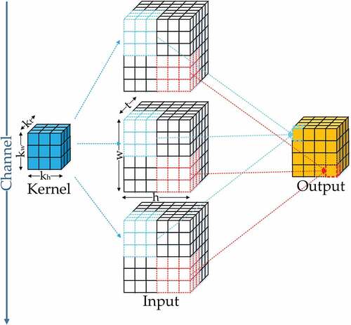
Figure 2. Comparison of (a) conventional convolution block and (b) multi-scale convolution block.
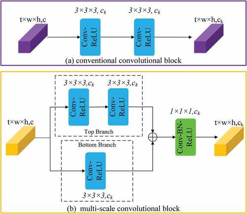
Figure 3. The receptive field of two stacked (3 × 3) convolution layers is equivalent to a (5 × 5) convolution layer.
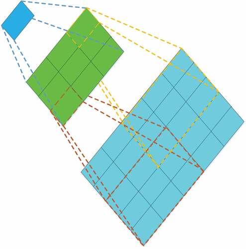
Figure 4. The structure of the Channel Attention Block (CAB).
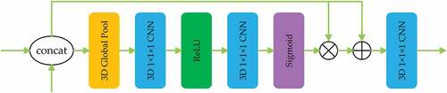
Figure 5. The structure of the Global Pooling Module (GPM).
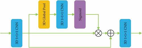
Figure 6. The structure of the proposed MSFCN network.
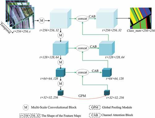
Figure 7. Examples of WHDLD images and their corresponding ground truth.
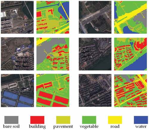
Figure 8. Examples of GID images and their corresponding ground truth.
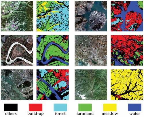
Figure 9. GF2 datasets gathered in (a) 2015, and (b) 2017. Each dataset owns four crop species labeled in different colors, and black pixels represent label information is absent. Patches indicated in red rectangles were utilized to train the network and the remainder to prediction.
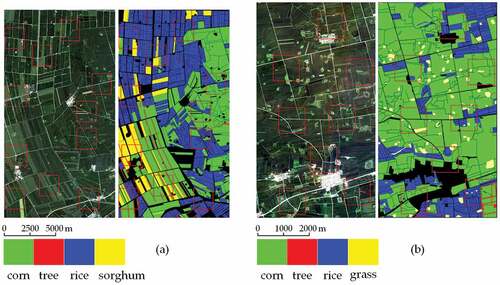
Table 1. The samples in WHDLD and GID datasets for each category for training, validation, and test
Table 2. The samples in 2015 and 2017 datasets for each category for training and test
Table 3. The experimental results on WHDLD and GID
Table 4. Per class F1-score performance on WHDLD and GID
Figure 10. Heat maps of different methods on (a) WHDLD and (b) GID.
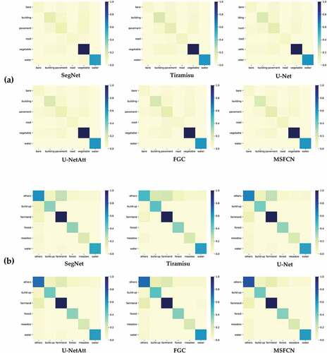
Figure 11. Land cover classification results of the method proposed and comparisons on (a) WHDLD and (b) GID.
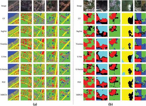
Table 5. The comparison of parameters and computational complexity for 2D datasets, where “M” is the abbreviation of million, the unit of parameter number, and “G” is the abbreviation of Gillion (thousand million), the unit of floating point operations
Table 6. The experimental results using different methods on 2015 dataset and 2017 dataset
Table 7. Per class F1-score performance on 2015 dataset and 2017 dataset
Table 8. The comparison of parameters and computational complexity for 3D datasets, where “M” is the abbreviation of million, the unit of parameter number, and “G” is the abbreviation of Gillion (thousand million), the unit of floating point operations
Figure 12. Heat maps of different methods on (a) 2015 and (b) 2017 datasets.
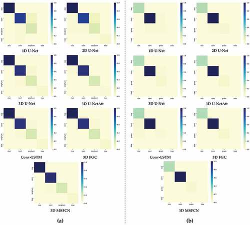
Figure 13. Land cover classification results of the method proposed and comparisons on the 2015 dataset and 2017 dataset, where the first three rows are from the 2015 dataset, and the remainder is from the 2017 dataset.
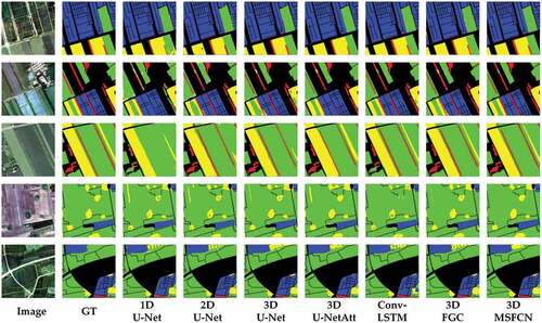
Table 9. The effectiveness of the Multi-Scale Convolutional Block and attention mechanisms on WHDLD and GID
Table 10. The comparison between the number of layers and the number of channels on the GID dataset
Table 11. The comparison of parameters and computational complexity for variants of MSFCN, where “M” is the abbreviation of million, the unit of parameter number, and “G” is the abbreviation of Gillion (thousand million), the unit of floating point operations
Data availability statement
The data used to support the findings of this study are included within the article.
WHDLD:https://sites.google.com/view/zhouwx/dataset?authuser=0#h.p_ebsAS1Bikmkd