
Figures & data
Figure 1. Workflow of the proposed population spatialization method.
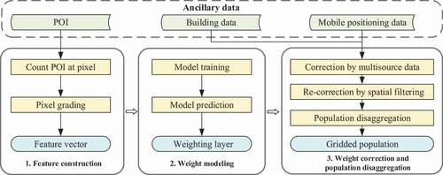
Figure 2. Illustration of cross-scale feature construction using POIs.
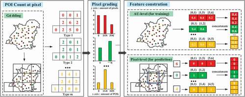
Figure 3. Flow of weight correction based on multi-source data.
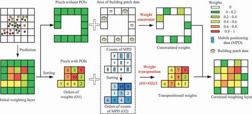
Figure 4. Overview of the study area Wuhan. (a) Location of Wuhan in Hubei Province. (b) Spatial distribution of 13 districts. (c) Spatial distribution of 186 streets with high, medium, and low population densities, respectively.
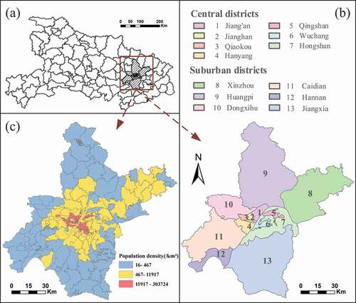
Table 1. Type, year, and source of experimental data.
Table 2. Types and counts of the selected POIs in experiments.
Figure 5. Accuracy comparison under an increasing numbers of grading levels at 500 m, 200 m, and 100 m resolutions, respectively.
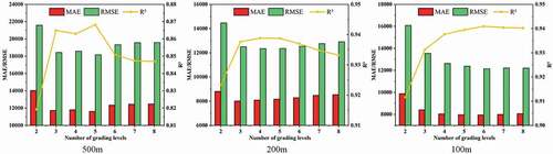
Figure 6. Accuracy comparison between CSFC method and TFC method. (a) The result at 500 m, 200 m and 100 m resolution, respectively. (b)-(c) Scatterplots of the predicted and the census population density at the street-level at 100 m resolution. A log10-log10 transformation was conducted for the population density. The red, green, and blue points represent high, medium, and low population density streets, while red, green, and blue line are fitting lines, respectively. The black dash line is the global fitting line.
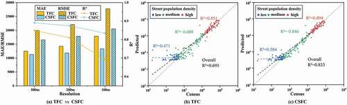
Figure 7. Variables importance for RF regression. The blue heatmap represents variables importance of 5 grading levels where the number of POIs in the pixel is from less to more accordingly for each POI type, while red heatmap represents the sum of variables importance of 5 grading levels.
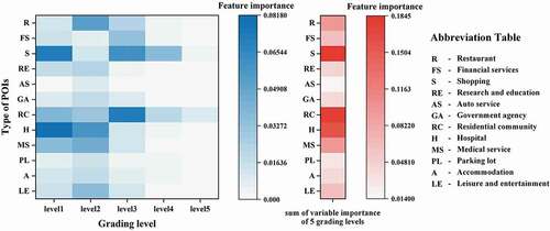
Figure 8. Accuracy comparison between weight correction method and traditional data fusion method (IVM). CSFC+WC represents the building patch data is used for Weight Constraint (WC) to correct the initial population weighting layer obtained from modeling based on CSFC, CSFC+WC+WT represents the further utilization of mobile positioning data for Weight Transposition (WT). (a) The result at 500 m, 200 m, and 100 m resolution, respectively. (b)-(c) Scatterplots of the predicted and the census population density at the street-level at 100 m resolution.
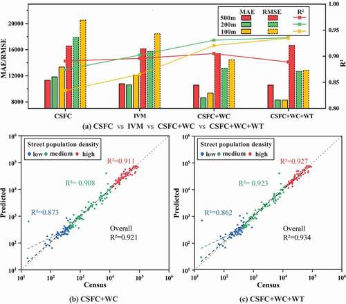
Figure 9. Accuracy comparison under different sizes of filtering template and different regions at 500 m, 200 m, and 100 m resolutions, respectively.
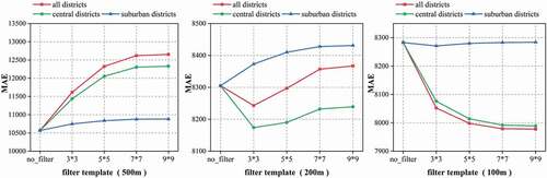
Table 3. Accuracies of GPW, WorldPop, Ye’s model and the proposed method at 500 m, 200 m, and 100 m resolutions, respectively.
Figure 10. Population spatialization results of our method at 100 m resolution and WorldPop dataset. For each amplified subregion, subgraphs (a) and (b) represents our results and WorldPop, respectively, while subgraphs (c) and (d) show the vector boundaries of Hangjiang River and Yangtze River in our results.
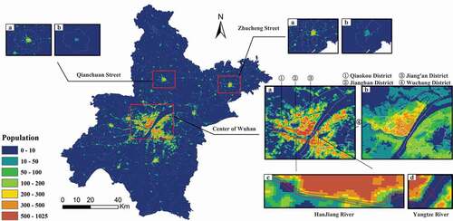
Figure 11. Accuracy comparison between our method, WorldPop and GPW at street-level. (a) -(c) Absolute error maps and accuracy histograms. (d)-(f) Relative error maps and accuracy histograms. (g)-(i) Scatterplots of the predicted and the census population density, and percentage histograms of the relative error.
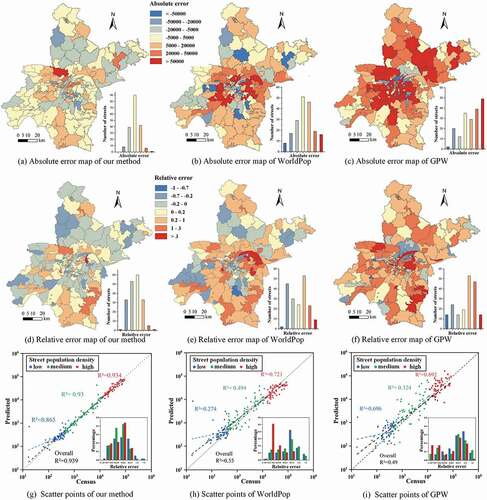
Table A1. The number and proportion of streets under different relative error ranges for three density levels.
Data availability statement
The code and data that support the findings of this study are openly available in GitHub at https://github.com/ZPGuiGroupWhu/PopulationSpatialization