A combined contour lines iteration algorithm and Delaunay triangulation for terrain modeling enhancement

Figures & data

Figure 1. (a) Level curves projected in a horizontal plane; (b) curve of steepest slope(James 2017).

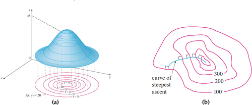
Figure 2. (a) Slopes of tangent lines on the surface; (b) the vertical plane passes through the direction of unit vector (James 2017).

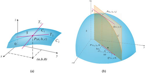
Figure 3. Gradient vector and tangent to the level curve are orthogonal vectors (James 2017).

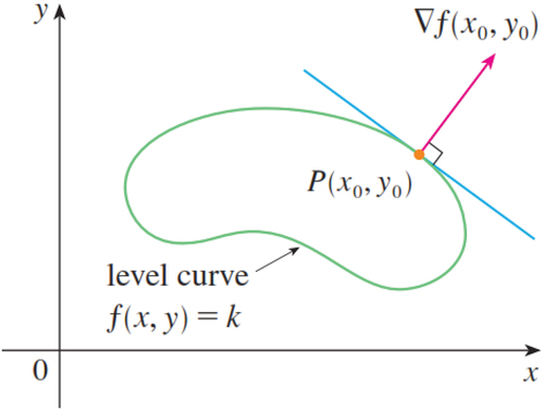
Figure 4. Flow chart of the proposed algorithm.

Table

Algorithm 1. Contour Lines Iteration Algorithm.

Input: contour lines extracted from 1:25,000 topographic map in a vector format, height values of spot points (m), initial contour interval value (m), the allowed ratio of false flat area as a percentage and symmetric differences area T (m^2). Output: DEM 1. Assigning elevation value for peak points. 2. Delineating orthogonal rays between contours. 3. Liner interpolation along the orthogonal rays using initial contour interval value. 4. Construction of intermediate contour lines. 5. Delaunay triangulation (TIN model) based on the intermediate contours concerning the associated contour interval. 6. False flat areas ratios estimation for the produced TIN models. 7. DEMs generation from the produced TIN models. 8. Generation of the contour lines from the DEM. 9. The process is repeated until obtaining a DEM that meets all predefined criteria.

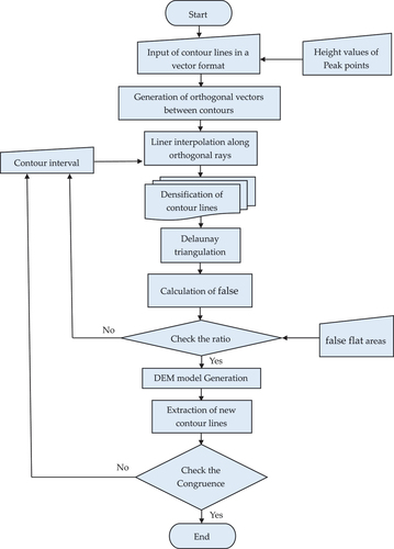
Figure 5. False flat area appeared due to the wrong distribution of triangles sides.

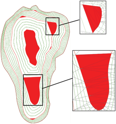
Figure 6. (a) The Orthogonal vectors based on four adopted methods (CAOV, CDOV, IAOV, IDOV) from left to right, (b) The intermediate contour lines extracted by linear interpolation along orthogonal vectors, (c) The new contour lines generated from TIN Models and the area in red color of false flat area, and (d) the symmetric differences between intermediate contour lines and newly generated contour lines.

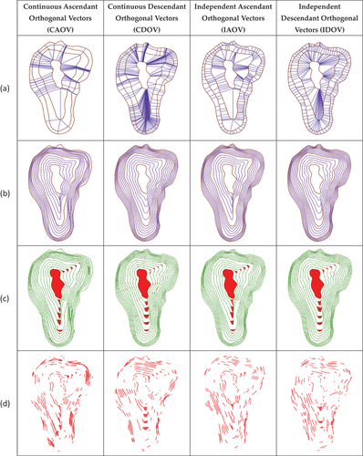
Table 1. Comparison between the statistics of tested methods.

Method Types	False flat Areas(%)	Interpolated Contours’ Symmetric Differences area (m^2)
CAOV	7.60	17,396
CDOV	7.78	7398
IAOV	7.36	3361
IDOV	7.61	4546

Figure 7. (a) The densification of level curves 0.5 m vertical interval，causing the generation of TIN model with 1.34% of false flat area (red regions), and (b) The densification of level curves 0.25 m vertical interval reduces the false flat area to 0.9%.

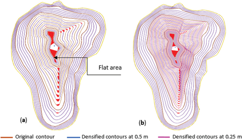
Figure 8. The examination samples of the study area according to three characteristic terrain locations, scale 1:25,000.

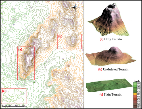
Figure 9. The precisions of TIN models as the increase of the intermediate contour lines.

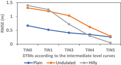
Table 2. The precisions of TIN models.

Digital terrain models	MAE (m)			RMSE (m)
	Plain	Undulated	Hilly	Plain	Undulated	Hilly
TIN0	0.77	0.97	1.04	0.67	1.31	1.40
TIN1	0.66	0.98	0.99	0.52	1.19	1.25
TIN2	0.56	0.89	0.77	0.41	1.03	0.72
TIN3	0.55	0.57	0.46	0.35	0.62	0.30
TIN4	0.50	0.48	0.17	0.26	0.29	0.05

Table 3. The geomorphometric parameters of DEMs and their statistics.

Parameter		Plain		Undulated		Hilly
		DTM4	TOPO raster	DTM4	TOPO raster	DTM4	TOPO raster
Altitude	Min.	324.25	318.91	397.25	396.79	368.99	368.94
	Mix.	359.41	360.01	492.18	490.56	540.81	540.50
	Mean	339.05	337.65	428.89	428.89	447.49	477.65
	S.D.	5.59	7.88	23.29	23.64	45.22	45.25
Local relief (m)	Min.	0.00	0.08	0.00	0.05	0.00	0.01
	Mix.	35.17	41.01	94.92	93.72	171.82	170.88
	Mean	14.82	18.74	31.69	32.41	78.52	79.03
Slope [°]	Min.	0.00	0.00	0.015	0.011	0.00	0.003
	Mix.	14.61	20.58	14.30	15.87	23.06	26.33
	Mean	0.81	1.02	3.0	2.99	6.10	6.09
	S.D.	0.87	1.41	2.27	2.37	3.86	4.01
Curvature [1/100 of m]	Min.	–2.07	–2.10	–1.89	–4.69	–3.49	–11.71
	Mix.	3.45	3.78	1.49	2.37	2.56	5.97
	Mean	–0.002	–0.003	0.00	0.004	0.002	0.011
	S.D.	0.095	0.097	0.139	0.124	0.352	0.329
Aspect [°] %	N (315^°-45^°)	12.55	14.63	4.47	4.31	11.30	10.76
	E (45^°-135^°)	11.01	12.83	31.28	30.17	21.27	20.94
	S (135^°-225^°)	37.96	34.00	27.21	27.82	20.59	19.98
	W (225^°-315^°)	38.48	37.68	37.04	36.88	46.84	47.50
	Flat area	0.00	0.86	0.00	0.82	0.00	0.82

Figure 10. Slope maps (a), (c), and (e) derived from DEM4, (b), (d), and (f) derived from TOPO raster DEM.

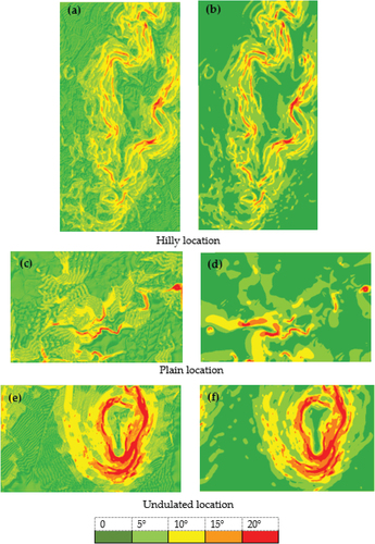
Figure 11. Curvature maps (a), (c), and (e) derived from DEM4, (b), (d), and (f) derived from TOPO raster DEM.

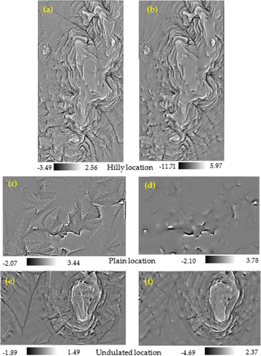
Figure 12. Aspect maps (a), (c), and (e) derived from DEM4, (b), (d), and (f) derived from TOPO raster DEM.

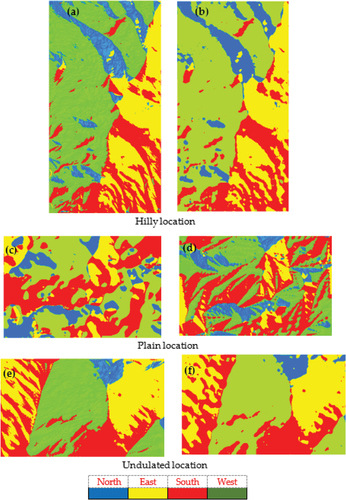
Figure 13. Spatial distribution of elevational changes between DEM4 and TOPO raster DEM (a) Hilly location; (b) Undulated location; and (c) plain location.

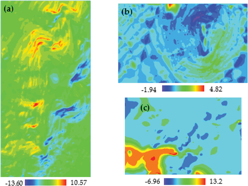
Figure 14. Comparison between original contour lines (brown color) and the generated ones (red color) from the extracted DEMs of the three types of terrain, line of maximum slope (blue color).

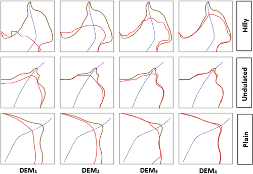
Figure 15. The convergence between extracted and original stream paths.

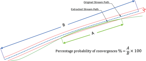
Table 4. Percentage probability of convergences between extracted and original stream paths.

DEMs according to the intermediate contour interval	Percentage probability of convergences (%)
	Plain	Undulated	Hilly
DEM0	70.28	62.30	66.28
DEM1	89.88	71.53	69.47
DEM2	93.63	83.39	73.75
DEM3	96.73	88.20	76.55
DEM4	96.91	94.93	84.03

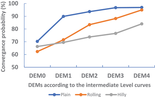
Figure 16. The convergence probability between extracted and original stream paths as the increase of the intermediate contour lines.

James, S. 2017. Calculus. Boston: Cengage Learning.

 Google Scholar

Data availability statement

The data that support the findings of this study are available from the corresponding author, upon reasonable request.