How do greenspace landscapes affect PM2.5 exposure in Wuhan? Linking spatial-nonstationary, annual varying, and multiscale perspectives

Figures & data

Figure 1. The study area and the spatial distribution of the 10 air quality monitoring sites (①-⑩) within Wuhan.

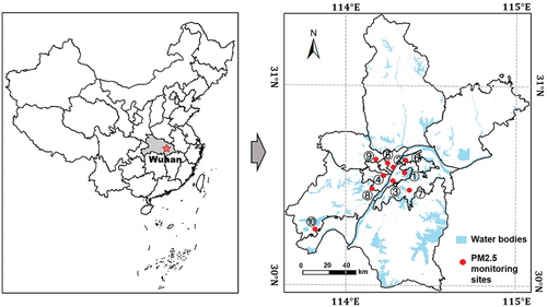
Figure 2. Spatial patterns of annual PM2.5 exposure (PW_PM2.5) across Wuhan from 2000 to 2016.

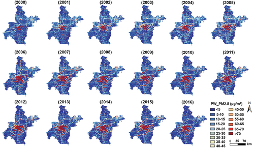
Figure 3. The time-series clustering results by K-DTW was shown in Figure 8(c). Spatial distribution of (a) inter-annual average, (b) standard deviation, and (c) time-series clustering result of PM2.5 exposure patterns in Wuhan in 2000–2016.

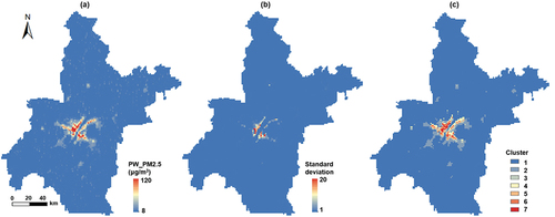
Figure 4. The average temporal variations of PM2.5 exposure risks in seven clusters and averaged across Wuhan from 2000 to 2016.

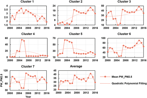
Table 1. The primary surface properties of seven time-series clusters.

Cluster No.	Primary surface properties
1	Mountainous forests and large-scale waterbodies, including the Yangtze River, the Hanshui River, the East Lake, the South Lake, and other large lakes.
2	Industrial estates (Wuhan Iron and Steel Cooperation) and built-up land that high intensively developed around 2006, including Zhuankou, Wujiashan, Nanhu, and Guanggu regions.
3	Junctures between built-up land and neighboring natural landscapes, including the beach of the Yangtze River located in Wuchang and Qingshan District, regions between Sha Lake and the East Lake, as well as Changfeng sub-district in Qiakou District.
4	Low/middle-rise high-density residential areas underwent significant renewal in 2004–2006, for instance, Wutaizha and Xujiapeng region in Wuchang, Yingwujie Qinduankou regions in Hangyang, as well as Dazhilu sub-district in Jianghan.
5	Middle/high-rise middle density residential areas without significant renewal after 2012, including the Jiyuqiao region in Wuchang, Yuehu region in Hanyang, and Beihu and Huaqiao sub-district in Jianghan and Jiang’an.
6	Middle/high-rise high-density residential areas are located in urban centers of Wuhan, and there was no remarkable change since 2006. This cluster generally includes Luonan and Shouyi sub-district in Wuchang, Hanzhengjie sub-district in Jianghan, Gutian, and Hanshuiqiao sub-district in Qiaokou.
7	It is mainly recognized as primary business areas and high-rise high-density settlements. In Jianghan and Jiang’an District, the coverage of this cluster extends from Baofeng to Xunlimen and Huangpu Road. In Wuchang District, this cluster mainly covers Simenkou, Zhongnan, Jiedaokou, and Xudong sub-centers.

Figure 5. Spatial distribution of PM2.5 exposure weighted barycenter in Wuhan from 2000 to 2016.

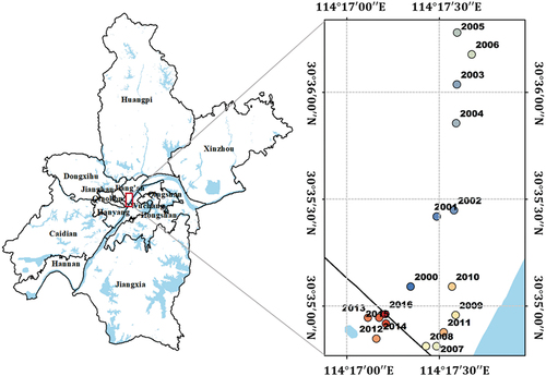
Figure 6. Spatial distributions of PM2.5 exposure hotspots in Wuhan from 2000 to 2016.

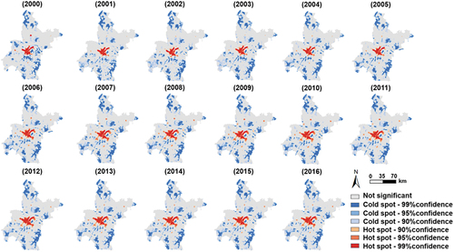
Table 2. Optimal bandwidths of GWR and MGWR from 2000 to 2015.

Variable	Model	2000	2005	2010	2015
Intercept	GWR	121	68	125	126
	MGWR	508	457	606	618
AI	GWR	121	68	125	126
	MGWR	258	192	267	271
ED	GWR	121	68	125	126
	MGWR	182	165	188	170
SI	GWR	121	68	125	126
	MGWR	94	86	101	105
PLAND	GWR	121	68	125	126
	MGWR	1570	1565	1612	817

Figure 7. Spatial distribution of local determination coefficient (Local R²) modeled by MGWR in the four years.

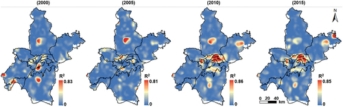
Figure 8. Regression coefficients of Aggregation Index (AI) from 2000 to 2015.

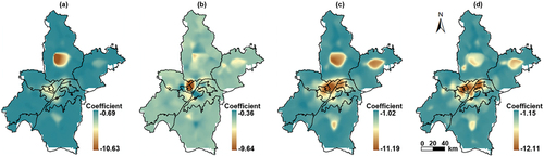
Figure 9. Regression coefficients of Edge Density (ED) from 2000 to 2015.

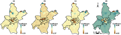
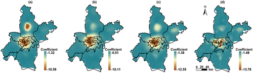
Figure 10. Regression coefficients of Shape Index (SI) from 2000 to 2015.

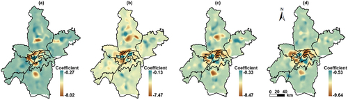
Figure 11. Regression coefficients of percentage cover of green spaces landscapes (PLAND) from 2000 to 2015.

Data availability statement

The annual ground-level PM2.5 concentration dataset can be accessed from the Socioeconomic Data and Application Center (https://beta.sedac.ciesin.columbia.edu/data/set/sdei-global-annual-gwr-pm2-5-modis-misr-seawifs-aod). The Landscan^TM population distribution data is provided by Oak Ridge National Laboratory (https://landscan.ornl.gov/). Annual land cover products in China (CLCD) are freely available at http://doi.org/10.5281/zenodo.4417810.