Estimating optimal substitution scale of urban gasoline taxis by electric taxis in the era of green energy: a case study of Zhengzhou City

Figures & data

Table 1. An example of taxi GPS trajectory for identifying serviced trips by taxi.

Vehicle ID	Timestamp	Longitude	Latitude	Speed	Direction	Service state	Trip
822022731	2018/7/1 9:59	113.XXXX	34. XXXX	48	0
822022731	2018/7/1 10:00	113.XXXX	34. XXXX	16	84	1	Start point
…	…	…	…	…	…	1
822022731	2018/7/1 10:35	113.XXXX	34. XXXX	22	356	1	End point
822022731	2018/7/1 10:36	113.XXXX	34. XXXX	28	356	0

Figure 1. The logic of ET simulation.

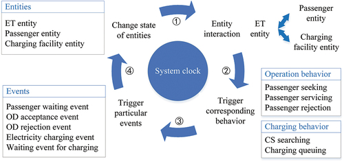
Figure 2. Simulation framework of ETs’ behavior.

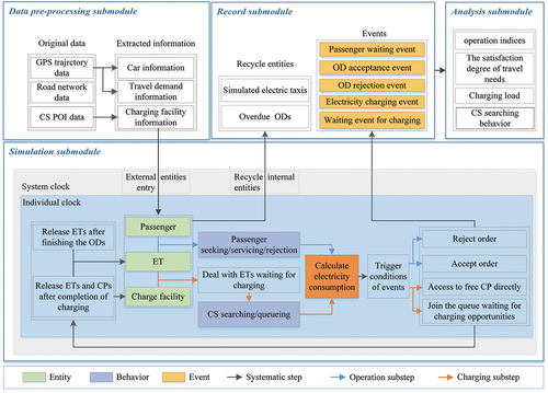
Table 2. Anxiety scale of the driver.

The degree of driver’s anxiety	$SOC$
No anxiety	>50% (Bi et al. 2017)
Anxiety	30%~50% (Bi et al. 2017)
Risky to shutdown	<30% (Bi et al. 2017)

Figure 3. Simulation flow chart of ETs’ operational behavior.

Figure 4. Simulation flow chart of CS searching behavior.

Figure 5. Simulation flow diagram.

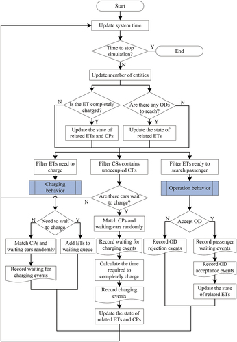
Figure 6. The changing regulation of $S_{ET}$ under different fleet sizes.

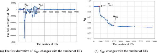
Figure 7. The changing regulation of $T_{wait}$ under different fleet sizes.

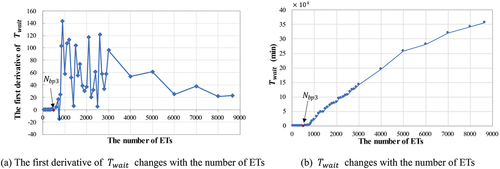
Table 3. Constant parameters in Equations (35)–(37).

Parameter	value
$e_{100}$	19.5 kW·h/100km
$M_0$	3 km (Liu 2020)
$i_0$	10 CNY (Liu 2020)
$i_1$	2 CNY/km (Liu 2020)
$Pric{e}_e$	1.5 CNY/kW·h (Liu 2020)

Figure 8. The changing regulation of $R_{ET}$ under different fleet sizes.

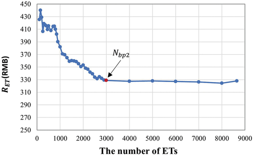
Figure 9. Study area and the road network.

Figure 10. Distribution of CSs.

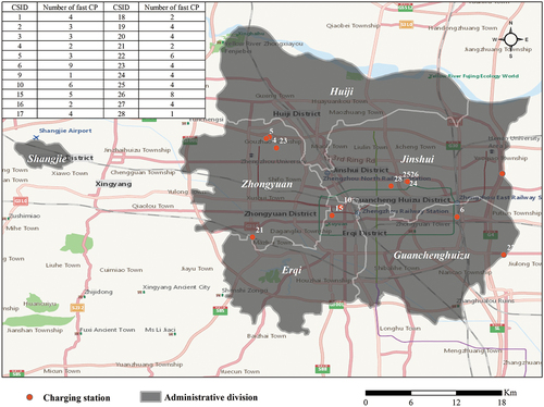
Table 4. Setting of parameters involved in the simulation program.

Parameters	Symbol	Values
Simulation start time	$T_s$	0:00
Simulation end time	$T_e$	23:59
Simulation time step	$t$	1 min
Driving range of ETs	M	240 km
ET power consumption of 100 km	$e_{100}$	19.5 kW·h
Charging power of CPs	P	30 kW
Waiting time threshold of Passengers	${\epsilon }_{wait}$	12 min
Adjustment coefficient of target $SOC$ for charging	k	0.75

Table 5. Parameters of the MOOP model derived from simulations.

Parameter	value	Parameter	value
$N_{bp1}$	800	$a_0$	−2.9e-03
$N_{bp2}$	3000	$b_0$	72.608
$N_{bp3}$	500	$c_0$	− 47,902
$\alpha$	−0.102	$a_1$	8e-06
$\beta$	1.6324	$b_1$	− 0.0622
$k$	−1e-06	$c_1$	439.71
$b$	0.8187	$k_1$	−3e-04
$\mu$	8e-16	$b_2$	328.84
$\sigma$	6.2366

Figure 11. Iteration of optimal substitution scale of taxi electrification.

Figure 12. Comparison of operation indices under different ET fleet sizes.

Figure 13. Division of traffic zones.

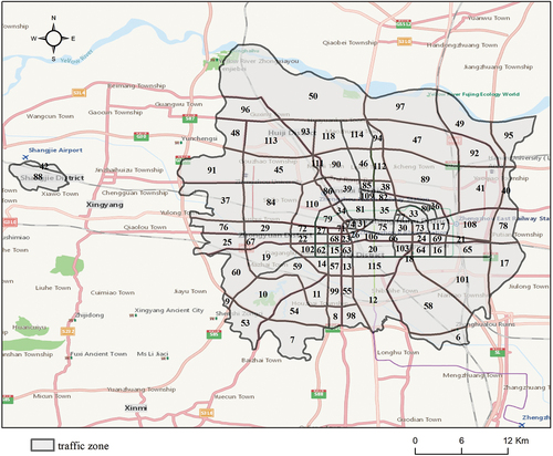
Figure 14. Temporal distribution of travel demands.

Figure 15. Spatial distribution of travel demands.

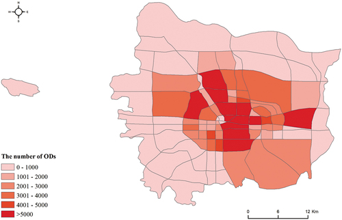
Figure 16. Spatial and temporal distribution of unmet travel demands.

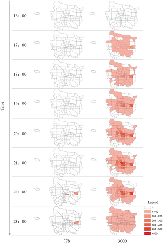
Figure 17. Distribution of business districts.

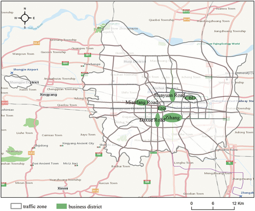
Figure 18. The usage of CSs under optimal substitution scenario and saturation substitution scenario.

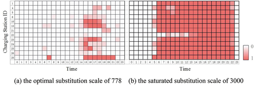
Figure 19. Css loads in temporal and spatial scales.

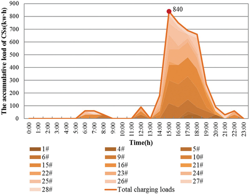
Figure 20. Frequency for each CS searching times in various electrification scale.

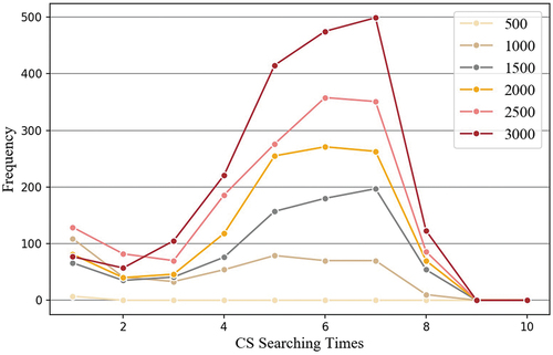
Figure 21. CS layouts from 2016 to 2020.

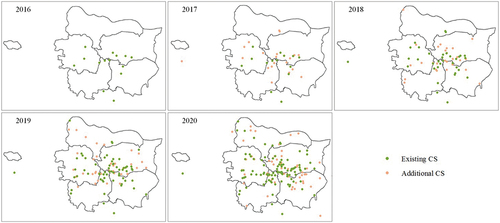
Table 6. The comparison of the quantity of charging facilities.

Time	The number of CSs	The number of CPs
2016	14	28
2017	36	72
2018	66	132
2019	106	212
2020	165	330

Figure 22. Iterations of OSS for 2016 to 2020 based on MOPSO algorithm.

Figure 23. The OSSs from 2016 to 2020.

Table 7. Parameters mentioned in the model.

Variables	Unit	Definition	Value
${\omega }_Q$	pax h/km	Distance cost factor	Equation (44)(44) ${\omega }_Q=\frac{Q_f+Q_m}{\mathrm{\Lambda }\ast P}$(44)
${\omega }_M$	pax h/h	Operating time cost factor	Equation (45)(45) ${\omega }_M=\frac{Q_{M0}+Q_{M1}}{\mathrm{\Lambda }\ast P}$(45)
${\omega }_Y$	pax h/site	Fixed CS cost factor	Equation (46)(46) ${\omega }_Y=\frac{Q_{Y0j}+Q_{Y1j}}{\mathrm{\Lambda }\ast P}$(46)
${\omega }_C$	pax h/port	Variable CS cost facto	Equation (47)(47) ${\omega }_C=\frac{Q_{C0j}+Q_{C1j}}{\mathrm{\Lambda }\ast P}$(47)
$Q_f$	CNY/[veh×km]	Fuel cost	0.14 (BK 2012)
$Q_m$	CNY/[veh×km]	Fleet maintenance cost	0.06 (Autohome 2018)
$Q_{M0}$	CNY/[veh×h]	Fleet depreciation cost	2.8 (HQEW 2016)
$Q_{M1}$	CNY/[veh×h]	Agency operating cost per time	12.36 (HQEW 2016)
$Q_{Y0j}$	CNY/[site×h]	Station installation fixed site cost	4.864
$Q_{Y1j}$	CNY/[site×h]	Station maintenance fixed site cost	2.432
$Q_{C0j}$	CNY/[site×h]	Station installation variable port cost	0.96
$Q_{C1j}$	CNY/[site×h]	Station maintenance variable port cost	0.486
$\mathrm{\Lambda }$	trips/h	Spatially homogenous peak-period pickup and drop-off demand	2
$GD{P}_p$	CNY/ppl×y	GDP per capita	78,003.73(GAOKAOHELP 2018)
$Q_{AWH}$	h	Average working hour annually	2300 (CNBS 2018)
$P$	CNY/pax h	Passenger value of time	Equation (48)(48) $P=\frac{GD{P}_p}{Q_{AWH}}$(48)
$M$	taxis	Number of taxis in the fleet	Equation (43)(43) $M=M_Q+M_E+M_C$(43)
$M_Q$	taxis	Number of taxis servicing trips	Equation (43)(43) $M=M_Q+M_E+M_C$(43)
$M_E$	taxis	Number of empty taxis	Equation (43)(43) $M=M_Q+M_E+M_C$(43)
$M_C$	taxis	Number of charging taxis	Equation (43)(43) $M=M_Q+M_E+M_C$(43)
$d$	km	Vehicle range for BEVs	240
$d_Q$	km	Expected distance traveled by a taxi while servicing a trip	7
$d_C$	km	Expected distance traveled by taxis while driving to a CS	Equation (49)(49) $d=N\left[d_Q+d_I\right]+2d_C$(49)
$d_I$	km	Expected distance traveled by a taxi while idle	Equation (49)(49) $d=N\left[d_Q+d_I\right]+2d_C$(49)
$T$	h	Expected cycle time	Equation (50)(50) $T=N\left[b_1+b_2+\frac{d_Q}{v}\right]+N\left[\frac{d_c}{Nv}+\frac{d_I}{v_I}\right]+\left[b_3+\frac{d_c}{v}\right]$(50)
$Y$	sites	Number of CS sites	85
$C$	ports	Number of CS ports	28
$k$		Routing factor	1.270
$D$	km	Length of the side of the square service region	32(HNPG 2018)
$N$	trips	Number of trips serviced between charging	$Nϵ\left[0,\frac{d}{d_Q}\right)$,
$v$	Km/h	Average speed traveled by taxis	28.5
$v_I$	Km/h	Speed traveled by an idle taxi	10
$b_1$	h	Boarding time	0.0042
$b_2$	h	Alighting time	0.017
$b_3$	h	Time spent at a CS by a taxi	1

Table 8. Optimal number of the reference model.

Empty-driving ETs	Passenger-carrying ETs	Charging ETs	Total number
9	209	57	295

Table 9. Comparison of the two solutions.

Empty-driving ratio (%)		Gasoline saved (L/d)		Utilization rate of CPs
Proposed approach	Reference model	Proposed approach	Reference model	Proposed approach	Reference model
54	10	11,018.7	4380.8	0.66	0.67

Bi, J., W. Zhang, X. Zhao, and T. Zhang 2017. “Charging Behavior Analysis of Electric Logistic Vehicle Based on Data Driven.” Journal of Transportation Systems Engineering 17 (1): 106–111. doi:10.16097/j.cnki.1009-6744.2017.01.016.

 Google Scholar

Liu, X.Y.D. 2020. “2021 Zhengzhou Taxi Fare Standard Adjustment Policy.” Accessed 5 August 2021. https://zz.bendibao.com/traffic/20201225/76676.shtm

 Google Scholar

BK. 2012. “How Much Does Byde6 Cost per Kilometer?” Accessed 15 November 2021. https://zhidao.baidu.com/question/385794817.html

 Google Scholar

Autohome. 2018. “How About the Maintenance Cost of Byde6?” Accessed 10 November 2021. https://club.autohome.com.cn/bbs/thread/fc1c66cf57c3ee6d/77326938-1.html

 Google Scholar

HQEW. 2016. Electric Taxi Charge Three Times a Day, Charging Inconvenience Constraints Development. Accessed 30 August 2021. https://tech.hqew.com/news_782418

 Google Scholar

GAOKAOHELP. 2018. “Henan’s per Capita GDP Ranking in 2018.” Accessed 27 September 2021. http://www.creditsailing.com/JingJiZhengCe/647365.html

 Google Scholar

CNBS. 2018. “China’s National Bureau of Statistics, China Works 9.2 Hours per Person, Almost the First in the World.” Accessed 27 September 2021. https://www.sohu.com/a/249636420_100176388

 Google Scholar

HNPG. 2018. “Henan People’s Government, Administrative Divisions of Zhengzhou.” http://www.henan.gov.cn/2006/09-08/231049.html. Accessed 30 September 2021.

 Google Scholar