Correlating fluency theory-based visual aesthetic liking of landscape with landscape types and features

Figures & data

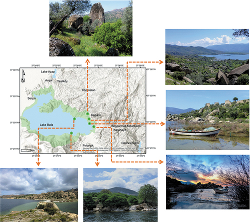
Figure 1. The geographical location of the study area and the historical sites.

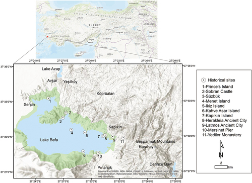
Table 1. Materials used in the study.

Materials	Source	Format
Geotagged photographs	Flickr and Google Earth	Point shapefile and.jgp files
Road data	OpenStreetMap	Polyline data
Digital Elevation Model (DEM)	NASA Earthdata	Raster data
Land uses map	Muğla Municipality	Polygon shapefile
Slope map	Generated from DEM	Raster data
Elevation map	Generated from DEM	Raster data

Figure 2. Methodology of the study.

Figure 3. Illustration of the image fluency metrics.

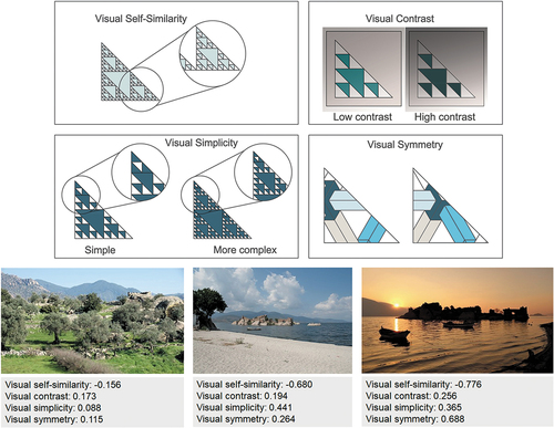
Figure 4. Sample landscape code.

Table 2. Classification of landscape features.

Landscape feature class	Description	Sample labels
Vegetation	Photographs showing trees, flowers, shrubs etc.	Tree, plant, scrublands, flower
Waterscape	Photographs illustrating lakes, rivers etc.	Lake, water, water resources
Geological feature/landform	Photographs depicting rocks, mountains etc.	Mountain, hill, highland, rock, bedrock, mountainous landforms
Historical landmark/architecture	Photographs depicting historical infrastructure (e.g. historical buildings, ruins)	Ruins, historic site, ancient history
Animal	Photographs focusing on animals such as birds, cows, donkeys etc.	Bird, cattle, donkey
Recreational facility/transportation	Photographs showing boats on Lake Bafa	Boat, vehicle
Built structure/human settlement	Photographs depicting buildings	House, chapel
Trail/path	Photographs illustrating roads, paths, trails	Road, trail

Figure 5. The spatial distribution of the geotagged photographs 2004–2020, types of road, and Euclidean distances.

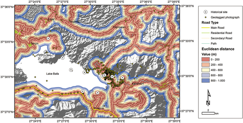
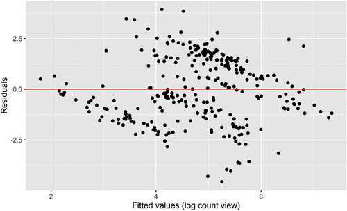
Table 3. Parameter estimates of the model (Std. Error: Standard error. Pr: probability. VIF: variance inflation factor. Time is the year the photograph was uploaded on Flickr.com. n = 284, + p < .10^.* p < .05^.** p < .01*** p < .001.).

Term	Estimates	Std. Error	t value	Pr(>|t|)	VIF
(Intercept)	3.13351	0.20880	15.007	<2e-16 ***	.
Contrast	−0.21744	0.10818	−2.010	0.0454 *	1.253171
Self-similarity	−0.12665	0.10542	−1.201	0.2306	1.190055
Simplicity	−0.58889	0.12692	−4.640	5.37e-06 ***	1.724806
Symmetry	0.15860	0.12920	1.228	0.2207	1.787404
Time	0.29424	0.03273	8.991	<2e-16 ***	1.024363

Figure 6. Viewshed analyses based on geotagged photographs with low, medium, and high levels of fluency.

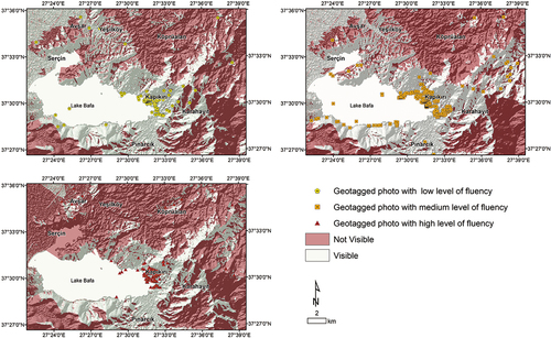
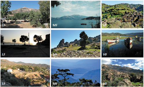
Figure 7. Spatial distribution of the types of landscape (l: low-altitude, m: medium-altitude, e: elevated, h: high-altitude, lo: low-gradient, me: medium-gradient, mo: moderate-gradient, hi: high-gradient, ag: agricultural areas, ar: artificial areas, ba: bare areas, bp: black pine forests, du: dunes, ft: treeless forest areas, ma: macchia, sp: stone pine forests, sw: swamps).

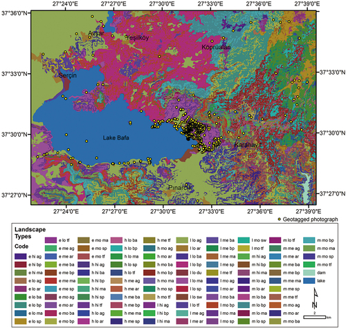
Table 4. Types of landscape by zone and level of visual aesthetic liking based on visibility analyses and unique landscape codes.

	Landscape types
	Near Zone (50 m)	Medium Zone (200 m)	Far Zone (1000 m)
High visual aesthetic liking	Medium-altitude, low-gradient artificial areas (m_lo_ar) High-altitude, moderate-gradient stone pine forests (h_mo_sp)	Medium-altitude, low-gradient artificial areas (m_lo_ar) High-altitude, moderate-gradient agricultural areas (h_mo_ag) Medium-altitude, moderate-gradient artificial areas (m_mo_ar)	Medium-altitude, low-gradient artificial areas (m_lo_ar) Medium-altitude, low-gradient stone pine forests (m_lo_sp) High-altitude, medium-gradient artificial areas (h_me_ar) High-altitude, moderate-gradient artificial areas (h_mo_ar) Medium-altitude, moderate-gradient artificial areas (m_mo_ar)
Medium visual aesthetic liking	High-altitude, high-gradient bare areas (h_hi_ba) Elevated, low-gradient artificial areas (e_lo_ar) Elevated, low-gradient treeless forest treeless (e_lo_tf) Medium-altitude, low-gradient macchia (m_lo_ma) Elevated, medium-gradient black pine forests (e_me_bp) Low-altitude, medium-gradient agricultural areas (l_me_ag) High-altitude, medium-gradient bare areas (h_me_ba) High-altitude, moderate-gradient black pine forests (h_mo_bp) Elevated, moderate-gradient treeless forest areas (e_mo_tf) Low-altitude, moderate-gradient swamps (l_mo_sw)	High-altitude, high-gradient bare areas (h_hi_ba) High-altitude, high-gradient black pine forests (h_hi_bp) Elevated, low-gradient artificial areas (e_lo_ar) High-altitude, low-gradient artificial areas (h_lo_ar) Elevated, medium-gradient bare areas (e_me_ba) High-altitude, medium-gradient stone pine forests (h_me_sp) Elevated, moderate-gradient artificial areas (e_mo_ar) Elevated, moderate-gradient bare areas (e_mo_ba)	High-altitude, high-gradient agricultural areas (h_hi_ag) High-altitude, high-gradient stone pine forests (h_hi_sp) High-altitude, low-gradient artificial areas (h_lo_ar) Elevated, medium-gradient bare areas (e_me_ba) Elevated, moderate-gradient bare areas (e_mo_ba)
Low visual aesthetic liking	Elevated, low-gradient bare areas (e_lo_ba) Low-altitude, moderate-gradient treeless forest areas (l_mo_tf) High-altitude, moderate-gradient treeless forest areas (h_mo_tf)	Elevated, high-gradient macchia (e_hi_ma)	Low-altitude, medium-gradient treeless forest areas (l_me_tf)

Figure 8. Binary heat map showing landscape features of geotagged photographs with high levels of fluency.

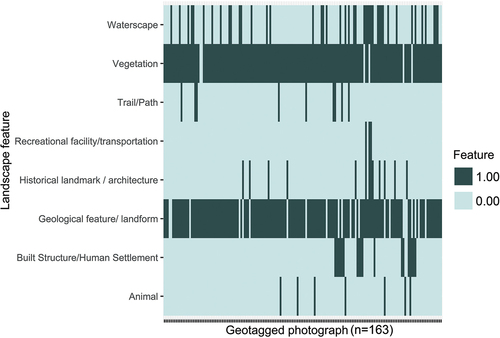
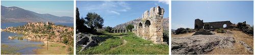
Figure 9. Photographs depicting ‘medium-altitude, low-gradient artificial areas’ (the ruins in the Kapıkırı village).

Data availability statement

There is no data related to this work.