Unravel the spatio-temporal patterns and their nonlinear relationship with correlates of dockless shared bikes near metro stations

Figures & data

Figure 1. The study area and the spatial distribution of metro stations in the main urban area of Wuhan.

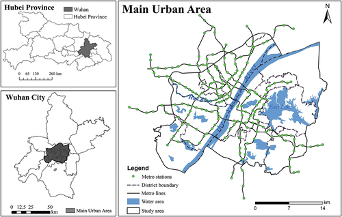
Table 1. Example of users’ records.

User_Id	Bike ID	Start-time	O_ longitude	O_ latitude	End-time	D_ longitude	D_ latitude
360550	26628	2019/11/2 20:38	114.4222	30.6058	2019/11/2 20:48	117.2631	34.81315
1012447	65287	2019/11/4 11:57	117.1335	36.6805	2019/11/4 12:11	117.1479	36.68504
980168	70546	2019/11/5 15:11	116.991	36.6689	2019/11/5 15:25	116.9819	36.66227

Figure 2. Schematic diagram of a service scope.

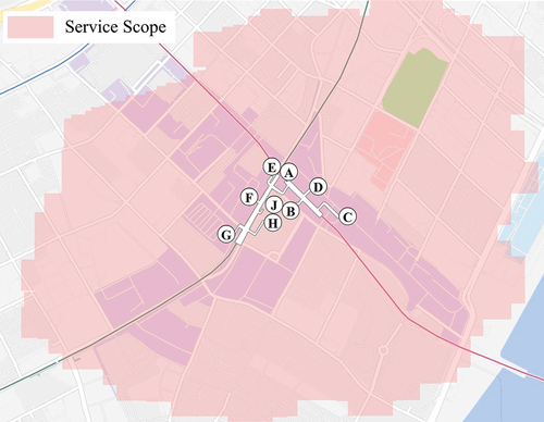
Figure 3. (a) Schematic diagram of inside flow, inflow, and outflow of a station; (b) Workday rhythm of $f_{total}$ and the corresponding spectrum diagrams of FFT; (c) Schematic diagram of convergence-divergence during a day.

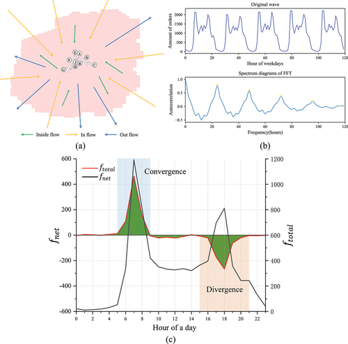
Table 2. Factors and collinearity diagnosis.

Variable	Name	Mean	St. dev.	VIF
Station attributes	Number of entrances	5.21	2.59	1.16
	Average distance of the nearest four stations (m)	1546.82	501.59	2.03
	Betweenness centrality	0.07	0.06	1.90
Demographics	BUD (per km^2)	6780.09	4011.18	6.11
	Resident density (per km^2)	2774.37	1579.63	4.12
	Employment density (per km^2)	3803.95	2883.24	5.18
	Job–housing ratio	1.85	2.03	1.94
Traffic conditions	Road density (km/km^2)	10.11	5.64	4.93
	Intersection density (per km^2)	11.23	7.42	4.09
	Bus station density (per km^2)	15.86	6.90	2.19
Land use variables	Shop density (per km^2)	6.61	5.70	5.63
	Living service facility density (per km^2)	60.09	55.78	5.57
	Commercial floor area ratio (%)	91.43	79.30	1.46
	Land use mix	0.60	0.11	1.58

Figure 4. Illustration of DTW distance: (a) Optimal path (black) between time series $S_1$ (red) and time series $S_2$ (blue); (b) a distance matrix showing the process of finding the optimal path and the DTW distance is the sum of distances (orange).

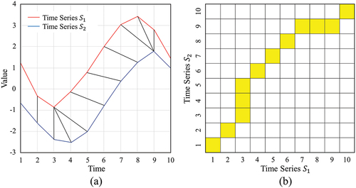
Figure 5. SSE and silhouette for different numbers of clusters (a) on weekdays (the elbow is at 6.) and (b) on weekends (the elbow is at 4.).

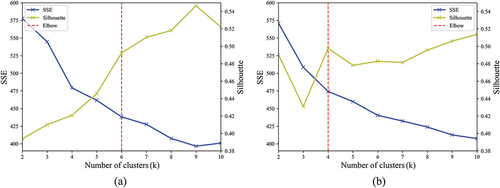
Table 3. Usage patterns for weekdays and weekends.

Clusters	LF-S	LF-CD	HF-DC	HF-CD	HF-S	HF-O
Weekdays	30.88%	22.79%	16.18%	13.24%	9.56%	7.35%
Weekends	55.15%	18.38%	-	18.38%	-	8.09%

Figure 6. Metro station distribution of different patterns and corresponding hourly profiles of $f_{total}$ (black) and $f_{net}$ (red) on weekdays.

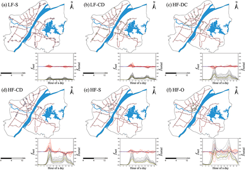
Figure 7. Hourly fluctuation of inside flow in different patterns on weekdays.

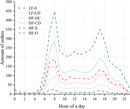
Figure 8. Metro station distribution of different patterns and corresponding hourly profiles of $f_{total}$ (black) and $f_{net}$ (red) on weekends.

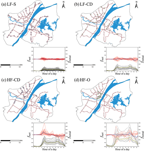
Figure 9. Hourly fluctuation of inside flow in different patterns on weekends.

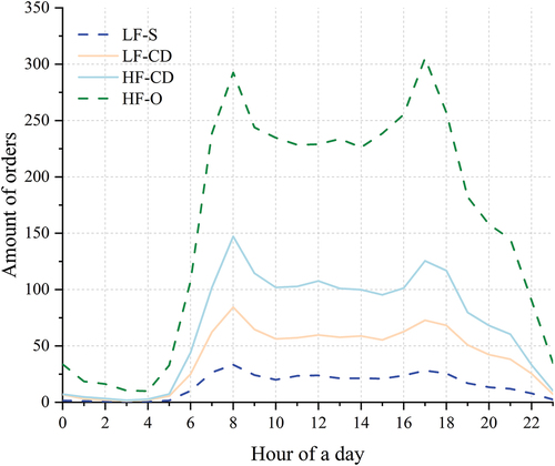
Table 4. Relative importance of variables.

Variable	Weekday		Weekend
	Relative importance (%)	Rank	Relative importance (%)	Rank
Station attributes	19.92		19.42
Number of entrances	7.62	5	6.49	10
Average distance of the nearest four stations	8.42	2	9.22	2
Betweenness centrality	3.88	14	3.71	14
Demographics	29.96		27.96
BUD	6.84	11	7.37	9
Resident density	7.40	6	7.79	6
Employment density	7.39	7	9.04	3
Job–housing ratio	8.33	3	3.76	13
Traffic conditions	23.78		27.15
Road density	9.50	1	10.69	1
Intersection density	7.04	10	8.90	4
Bus station density	7.24	8	7.56	8
Land use variables	26.34		25.47
Shop density	7.14	9	7.65	7
Living service facility density	7.80	4	8.36	5
Commercial floor area ratio	5.59	13	4.13	12
Land use mix	5.82	12	5.32	11

Figure 10. Nonlinear associations between the top five key variables and usage patterns on weekdays.

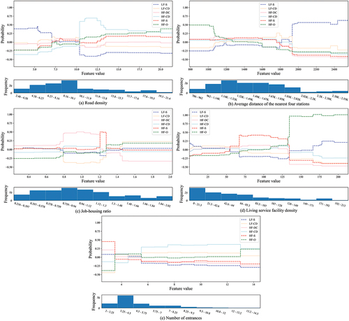
Figure 11. Nonlinear associations between the top five key variables and usage patterns on weekends.

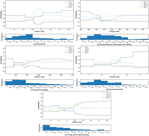
Figure 12. Hourly fluctuation of bike-sharing demand per day.

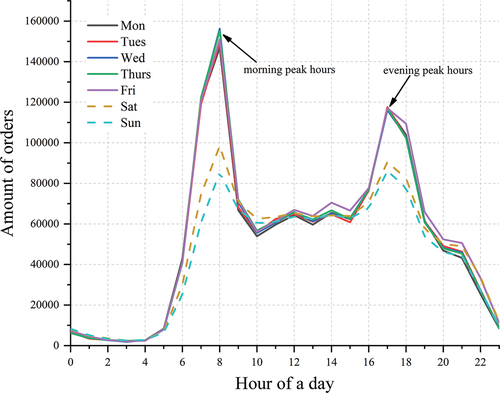
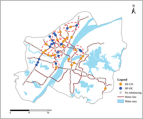
Figure 13. Dynamic rebalancing zones adjacent to HF-CD pattern and HF-DC pattern inside the red ellipse.

Data availability statement

Restrictions apply to the availability of these data. The data are not publicly available due to Mobike’s contract and privacy policy.