
Figures & data
Figure 1. Proposed flowchart for transforming coordinates of points from WGS84 to ITRF.
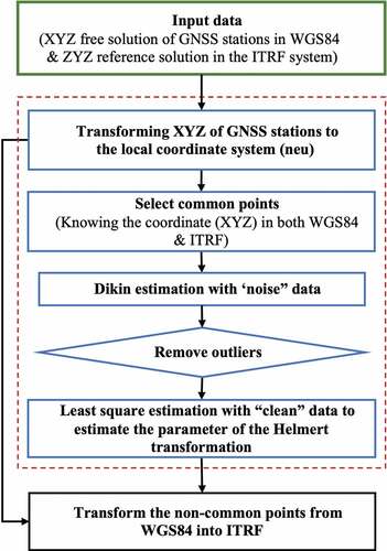
Figure 2. Helmert transformation between two 3D coordinate systems.
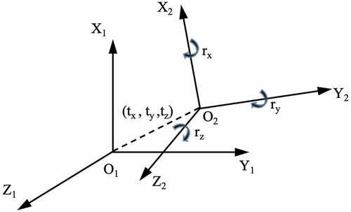
Figure 3. Global coordinate system and the local coordinate system.
Figure 4. Example of LS and robust estimation (Press et al. Citation1992).
Figure 5. The common points of the Géoazur GNSS network.
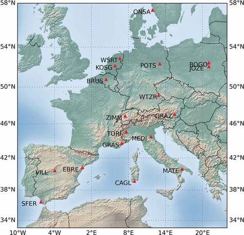
Table 1. Coordinates of 18 common points in WGS84 and ITRF at the 1998.0055 epoch.
Table 2. Residuals of common points estimated by the LS estimation with “noisy data”.
Table 3. Residuals of common points estimated from the Dikin estimator with “noisy” data.
Table 4. Residuals of common points estimated by the LS estimation with “clean” data.
Table 5. Comparison of estimated Helmert transformation parameters by the least square estimation and robust estimators (ppb stands for part per billion and mas stands for milliarcsecond).
Table 6. Comparison between estimated Helmert transformation parameters of classical LS and WTLS estimation.
Data availability statement
Some or all data, models, or code that support the findings of this study are available from the corresponding author upon reasonable request:
− Code of Helmert transformation Programe by Python.
− Free solution of Géoazur GNSS network at epoch 1998.0055.
− Reference solution of ITRF2012 IGS12P33.snx
- Discontinuity solution of ITRF2012 sonl_2012.snx