A comparative analysis of grid-based and object-based modeling approaches for poplar forest growing stock volume estimation in plain regions using airborne LIDAR data

Figures & data

Figure 1. Spatial patterns of poplar distributions in plain regions.

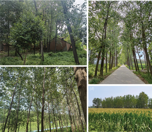
Figure 2. The study areas Lixin County and Yongqiao District in Anhui Province, China: (a) shows topography of Anhui Province by digital elevation model (DEM), (b) and (c) show spatial distributions of poplar species with sample plots in Yongqiao and Lixin, respectively.

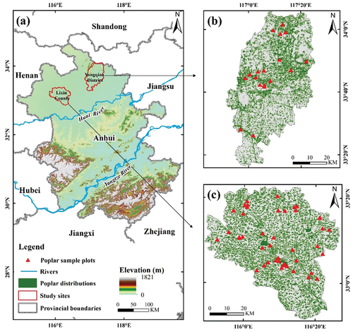
Figure 3. Framework for developing poplar forest growing stock volume (GSV) estimation models based on airborne LIDAR and Gaofen-6 data.

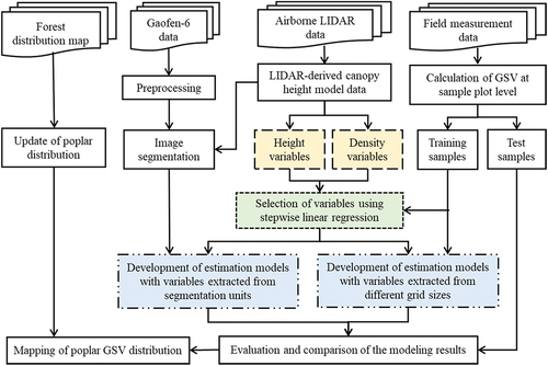
Table 1. The datasets used in this study.

Datasets	Acquisition dates	Descriptions
Field measurements	June–September 2019	Sample plot size of 25.82 m by 25.82 m
Airborne LIDAR	June 2019	Point density of over 2 point/m^2
Gaofen-6 imagery	9 July 2019	Panchromatic image with a spatial resolution of 2.1 m and multispectral images of 4 bands with a spatial resolution of 8 m
Forest map	2019	Forestland “One Map” in vector format

Table 2. The DBH and GSV statistics of poplar sample plots.

Study areas	Number of sample plots	DBH (cm)			GSV (m^3/ha)
		Range	Mean	Standard deviation	Range	Mean	Standard deviation
Linxin	43	5.00–58.00	17.98	7.33	51.60–175.31	117.96	27.95
Yongqiao	18	5.20–61.80	16.95	8.06	19.45–183.65	118.45	53.02

Table 3. Poplar GSV estimation models using LIDAR CHM-derived variables at a plot size of 26 m × 26 m.

Study areas	Predictive variables	GSV estimation model fitting		Model validation
		Linear models	R^2fit	R^2	RMSE (m^3/ha)	RMSEr (%)
Lixin	Height	−32.71 + 7.74H85	0.50	0.46	20.23	17.15
	Height & Density	−26.28 + 13.31H10 + 6.07H85 − 2.86D4 + 3.12D7 − 5.62D9 + 4.18D10	0.76	0.71	14.94	12.67
Yongqiao	Height	−24.71 + 8.46H70	0.92	0.89	16.59	14.50
	Height & Density	Same as the model with height variables		Same as the model with height variables

H_i is the ith height percentile; D_j is density at the jth layer.

Figure 4. Relationships between the predicted poplar growing stock volume using developed models and observed values of sample plots, including the scatter plots in Lixin which the models were developed using canopy height variables (a1) and a combination of canopy height variables and density variables (a2); the scatter plot in Yongqiao which the model was developed using canopy height variables only (b).

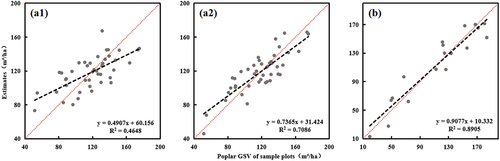
Table 4. Summary of GSV estimation accuracy assessment results based on different scenarios.

Study areas	Statistical unit (m^2)		GSV estimation models	R^2fit	Model validation
					R^2	RMSE (m^3/ha)	RMSEr (%)	Bias (m^3/ha)
Lixin	Grid-based	10 × 10	−2.63 + 6.245H90	0.52	0.48	19.88	16.85	4.29
		15 × 15	−17.37 + 6.82H90	0.56	0.53	18.90	16.02	3.02
		20 × 20	−23.35+7.34H85	0.58	0.54	18.68	15.84	3.16
		20 × 20	−77.35+10.78H10+8.43H85 +2.24D7$-$3.33D9	0.78	0.74	14.02	11.89	1.62
		26 × 26	−26.28+13.31H10+ 6.07H85+4.18D10 $-$5.62D9$-$2.86D4+ 3.12D7	0.76	0.71	14.94	12.67	14.75
	Object-based		−39.87 + 7.53H90	0.61	0.56	13.82	11.66	4.88
Yongqiao	Grid-based	10 × 10	−18.92 + 7.40H80	0.88	0.86	18.73	16.37	−2.46
		15 × 15	−24.46 + 7.75H85	0.90	0.88	16.79	14.67	−2.48
		20 × 20	−18.15 + 8.02H70	0.91	0.90	15.99	13.97	−0.65
		26 × 26	−24.72 + 8.46H70	0.92	0.89	16.59	14.50	−4.04
	Object-based		−24.64 + 9.17H60	0.91	0.90	15.84	13.85	0.01

H_i is the ith percentile of canopy height; D_j is density at the jth layer.

Figure 5. Relationships between observed poplar GSV of sample plots and estimated GSV based on different scenarios: (a1) to (a4) represent the statistical units at which the variables were extracted 10 m × 10 m, 15 m × 15 m, 20 m × 20 m, and segment, respectively in Lixin, (b1) to (b4) represent the same statistical units in Yongqiao.

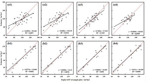
Figure 6. The growing stock volume estimates at segments (a) and (c) and grid sizes of 20 m × 20 m (b) and (d) in Lixin and Yongqiao ((a) and (b) for Lixin; (c) and (d) for Yongqiao).

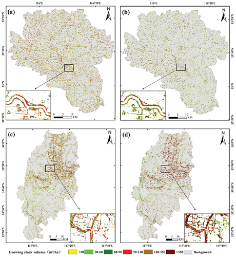
Figure 7. Poplar growing stock volume estimates of typical poplar strip forests from grid-based and object-based approaches: (a1) and (a2) represent grid-based estimates based on grid size of 20 m × 20 m and object-based estimates in Lixin, (b1) and (b2) represent grid-based object-based estimates in Yongqiao.

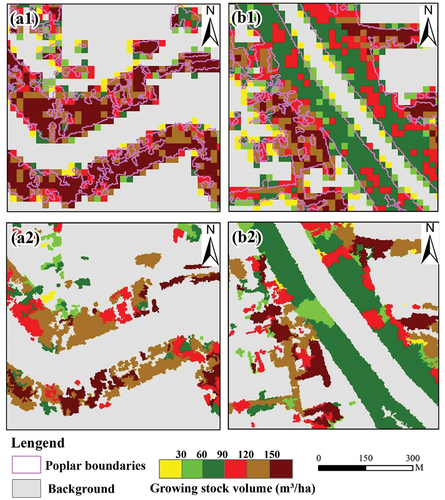
Table 5. A comparison of estimated total GSV amounts in both study areas.

Study area	Grid-based calculation		Object-based calculation		GSV rate (%)	Area rate (%)
	GSV (×10^6 m^3)	Area (ha)	GSV (×10^6 m^3)	Area (ha)
Lixin	1.9631	30952.04	1.2628	16949.01	55.46	82.62
Yongqiao	2.0076	25504.28	1.7672	20549.35	13.60	24.11

Figure 8. A comparison of scatter plots based on the GSV estimates from grid-based (20 m × 20 m) and object-based modeling approaches in Lixin ((a), (b) are based on the combination of CHM metrics and density variables; (c), (d) are based on CHM metrics only; (a), (c) include fully covered poplar plots while b, d include partially covered poplar plots) and Yongqiao ((e) means fully covered poplar plots, (f) means partially covered poplar plots).

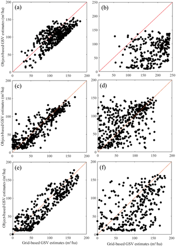
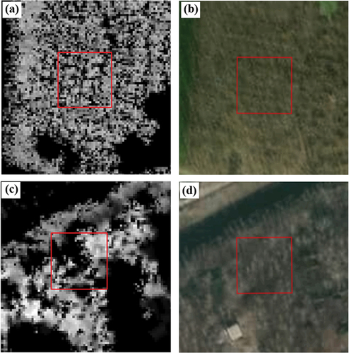
Figure 9. Two poplar sample plots from Yongqiao ((a) and (b)) and Lixin ((c) and (d)) showing the differences in poplar stand structures from LIDAR CHM ((a) and (c)) and high spatial resolution images ((b) and (d)).

Data availability statement

Due to confidentiality agreements, supporting data can only be made available to bona fide researchers subject to a nondisclosure agreement. Details of the data and how to request access are available from Professor Dengsheng Lu at Fujian Normal University.