
Figures & data
Figure 1. The flowchart and conceptual illustration include the input data and processing (a), extract TLP considering the road characteristics (b), and the calculation of join weights (c).
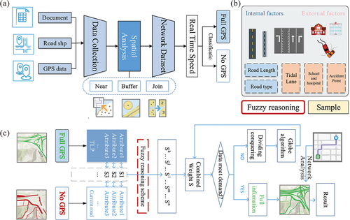
Table 1. National speed limits of UK road.
Figure 2. Classification and types of roads in England (a), road speed limits stipulated by the Department for Transport (b), and GPS speed distribution of different classifications (c) and types (d) of roads. The colors of the boxplot correspond to the road speed limit colors (b), and the violin plot colors correspond to the classification of UK roads (a).
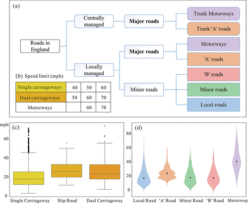
Figure 3. Similarity curve: Bell-shaped (a), S-shaped (b) and Z-shaped (c).
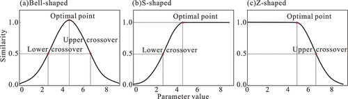
Figure 4. Conceptual illustration of similarity calculation. Left column shows a 5-dimensional similarity vector illustration. The right column shows examples of similarity and speed calculations.
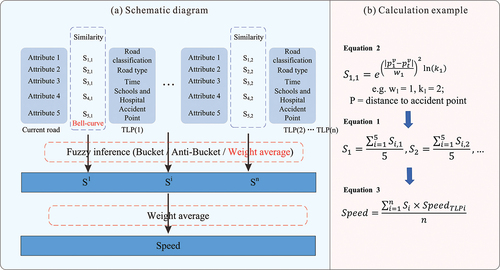
Figure 5. Conceptual illustration of attributes similarity between link and TLP. First, calculate the similarity of attributes space considering infrastructure and accident point factor (a). Then calculate the road classification’s similarity between links and TLP (b), judging the type and period of the road through the values of yes and no (c). Finally, the n-dimensional vector’s similarity is acquired for all TLPs, representing the link and its comprehensive characteristics.
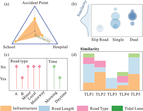
Figure 6. Conceptual illustration of barrel theory, anti-barrel theory and weighted average.
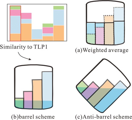
Figure 7. The whole link is divided into sub-links (a) and sub-links into whole link (b).
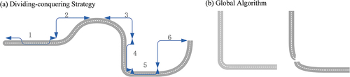
Figure 8. Map of the road network (blue line) distribution in Newcastle, the dotted line represents the border of Newcastle.
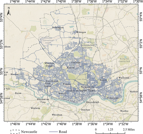
Table 2. Data used in this work.
Table 3. Data used in this work.
Figure 9. Scatterplots between observed GPS speed (y-axis) and fuzzy inference predicted average link road speed (x-axis). The red line represents the linear regression fit.
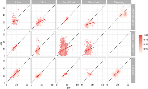
Figure 10. Observed GPS speed (y-axis) and fuzzy inference predicted average link road speed (x-axis) scatterplots in morning (a) and daytime periods.
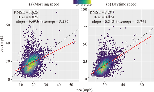
Figure 11. Cross-validation results. First, calculate the average speed for each road type and classification (a), then compare observed versus predicted for all road link speeds (b).
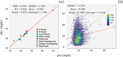
Table 4. Sample selection categories and data statistics.
Figure 12. The results of the first group of tests select different time periods and carry out comparative experiments. Static (a) and fuzzy impedance models (b-c) routing results comparison in daytime and morning.
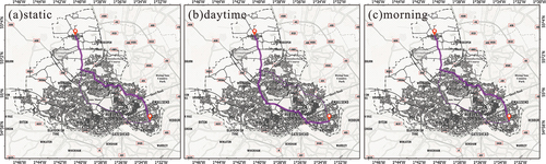
Table 5. Comparison of statistical indexes on static and fuzzy impedance models.
Figure 13. The results of the second group of tests select daytime periods and carry out comparative experiments. Static (a1, b1) and fuzzy impedance models (a2, b2) routing the results comparison in the daytime.
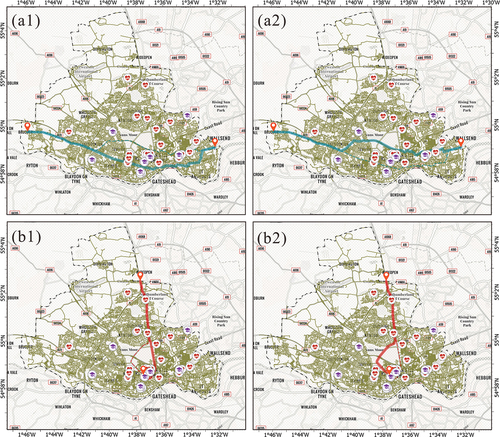
Table 6. Comparison of statistical indexes on static and fuzzy impedance models.
Data availability statement
Data will be made available on request.