Figures & data
Figure 1. Study area, including gravel pit ponds (bright blue) and the boundary of the PRSE (black).
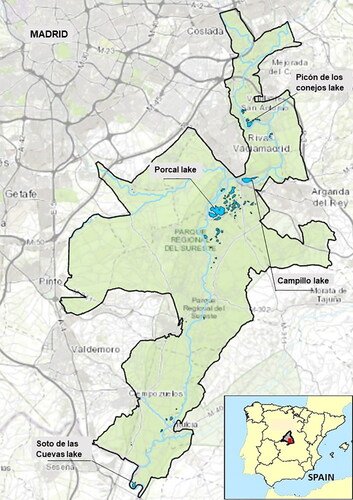
Figure 2. Picón de los Conejos lake development from 1987 to 2011, with the assumed shape in this study (light blue dashed line).
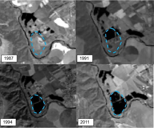
Figure 3. Campillo lake development from 1984 to 2011, with the assumed shape in this study (light blue dashed line).
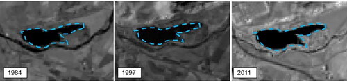
Figure 4. Porcal lake development from 1984 to 2011, with the assumed shape in this research (light blue dashed line).
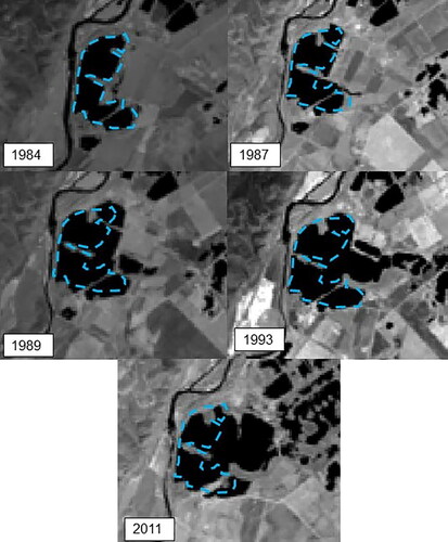
Figure 5. Soto de las Cuevas lake development from 1984 to 2011, with the assumed shape in this research (light blue dashed line).
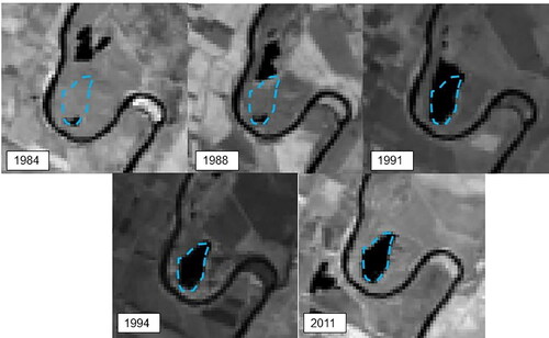
Figure 6. Flow chart of the research process.
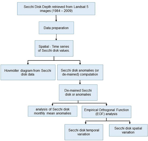
Table 1. Evaluated MICE library methods.
Figure 7. Overview of the time series analysis of variables using the temporal and spatio-temporal approaches.
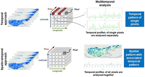
Figure 8. Hovmöller diagrams for (a) Picón de los Conejos; (b) Porcal; (c) Campillo and (d) Soto de las Cuevas lakes.
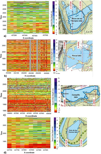
Figure 9. Secchi disk annual means for each gravel pit pond and trophic OECD classifications.
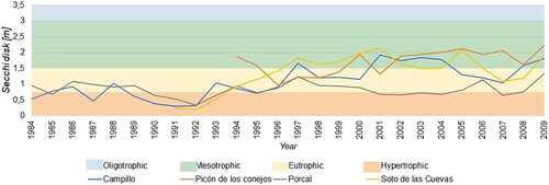
Figure 10. (a) Monthly evolution of Secchi disk anomalies; b) box plot with the mean (blue points), minimum, maximum, median, first quartile, and third quartile.
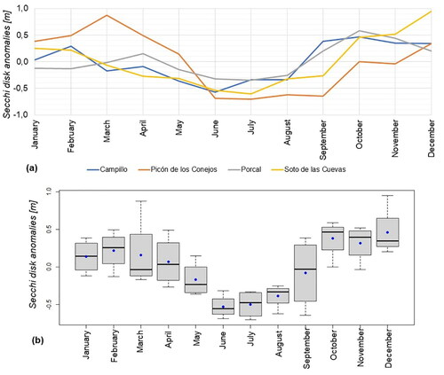
Figure 11. Monthly evolution of Secchi disk Picón de los Conejos anomalies compared with (a) air temperature and (b) global radiation.
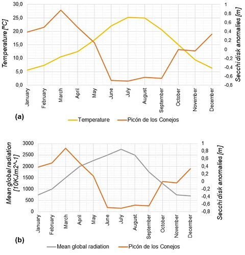
Figure 12. Monthly spatial evolution of Secchi disk anomalies in the Campillo water pit pond.
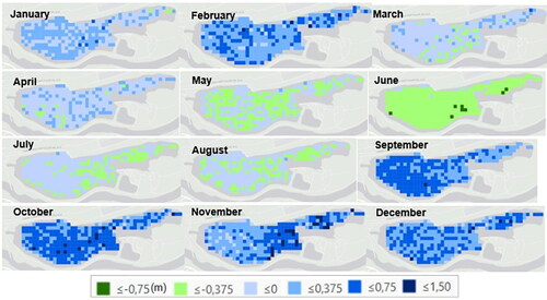
Figure 13. Magnitude of change of the Secchi disk for each pixel throughout the studied time series (1984–2009) for (a) Picón de los Conejos; (b) Porcal; (c) Campillo and (d) Soto de las Cuevas lakes.
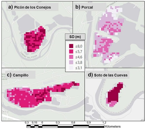
Figure 14. Mode 1 spatial variability of EOF analysis for (a) Picón de los Conejos; (b) Porcal; (c) Campillo and (d) Soto de las Cuevas lakes.
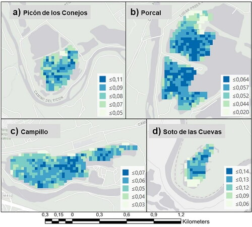
Figure 15. Mode 1 temporal variation of EOF analysis for (a) Picón de los Conejos; (b) Porcal; (c) Campillo and (d) Soto de las Cuevas lakes; the date where the year is located corresponds to May 1 for each year.
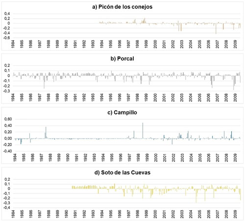
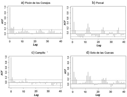
Figure 16. Autocorrelation function of temporal variation mode 1. (a) Picón de los Conejos; (b) Porcal; (c) Campillo and (d) Soto de las Cuevas lakes.