Using multisource satellite products to estimate forest aboveground biomass in Oita prefecture: a novel approach with improved accuracy and computational efficiency

Figures & data

Figure 1. (a): Location of study area with land use and land cover classification. (b): Distribution pattern of DBF (c): Proportion of landscape. DBF: deciduous broadleaf forest, DNF: deciduous needleleaf forest, EBF: evergreen broadleaf forest, ENF: evergreen needleleaf forest. (d): SRTM DEM. (e): PALSAR-2 L-band SAR image displayed as RGB = HV, HH, VH in db. (f): Sentinel-1 C-band SAR image displayed as RGB = VV, VH, VV in db. (g): Sentinel-2 MSI image in true color composite (RGB = Red, Green, Blue).

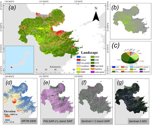
Figure 2. Research flow.

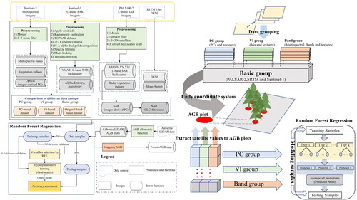
Figure 3. Airborne LiDAR Data. (a) example of modelling data, (b) close-up of airborne LiDAR plots, (c) Oita prefecture.

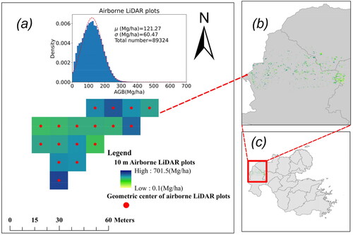
Table 1. Summarize of satellite derived variables.

Dataset	Dates (yyyy.mm.dd)	Variables Groups	Descriptions
Sentinel-2(S2)	2020.04.06	Multispectral bands	2, 3, 4, 5, 6, 7, 8, 8A, 11, 12
		Vegetation indices	NDVI (Rouse et al. 1974), EVI (Huete et al. 2002), GARI (Gitelson et al. 1996), GCI (Gitelson et al. 2003), GDVI (Sripada 2005), GNDVI (Gitelson and Merzlyak 1998), GRVI (Sripada et al. 2006), SAVI (Huete 1988), SR (Birth and McVey 1968) and DVI (Tucker 1979)
		PCA bands	Multispectral bands derived PCA bands
		Relative Textures from multispectral bands, VIs, and PCs	Contrast, Dissimilarity, Homogeneity, Second Moment, Energy, Max Probability, Entropy, Mean, Variance and Correlation
Sentinel-1(S1)	2020.06.10	C-Band Polarization channels	VV, VH
		Polarization decomposition	Entropy, Anisotropy, Alpha
PALSAR-2	2020.08.01,2020.08.15, 2020.09.03,2020.09.17,	L-Band Polarization channels	HH, HV, VV, VH
		Radar indices	I1 (Kim et al. 2011), I2 (Huggannavar and Shetty 2020), I3 (Huggannavar and Shetty 2020)
		PCA bands and relative textures	L-Band Polarization channels derived PCA bands and its relative textures
SRTM		Topographic parameters	Elevation, Slope, Aspect

Table 2. Summarize of regression models.

RF-based model	Description	Total number of input features
PCA-model	Basic data, 3 PCs, and 30 relative textures.	70
VI-model	Basic data, 10 VIs, and 30 related textures.	77
Band-model	Basic data, 10 original bands, and 30 related textures.	77
All data	Basic data, 3 PCs, 10 VIs, and, 10 original bands, 90 related textures.	150

Figure 4. Result of PCA, the selected bands are pointed in red. (a): Sentinel-2 Multispectral Bands. (b): PALSAR-2 Polarized Channels.

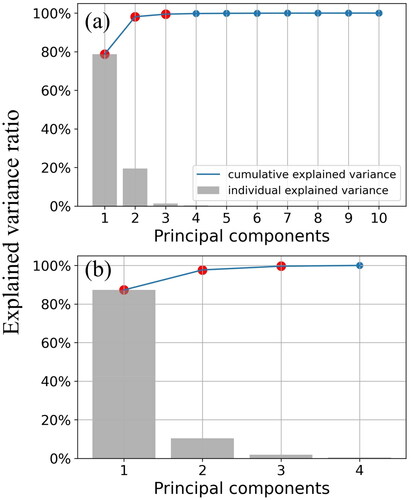
Figure 5. Coefficient matrix between AGB and Variables. (a) Bands (b) VIs.

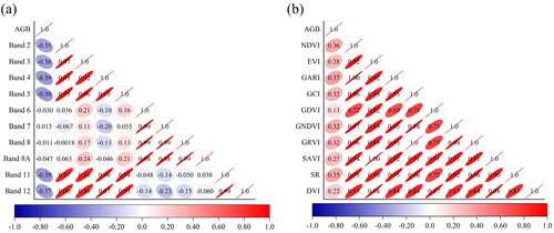
Figure 6. Result of RFE, the best result case of each model is indicated by black node.

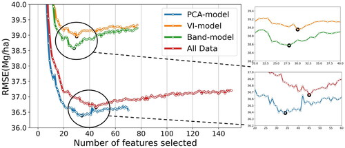
Figure 7. Observed and predicted AGBs for testing samples: (a) PCA-model, (b) VI-model, (c) Band-model, (d) All data; The 1:1 line is marked by the dashed black lines.

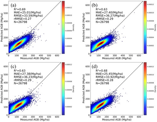
Figure 8. Variables listed in order of importance based on Gini importance: (a) PCA-model, (b): VI-model, (c): Band-model, (d): All data; abbreviation: S2: Sentinel-2, S1: Sentinel-1, P: PALSAR-2, others in Table 1.

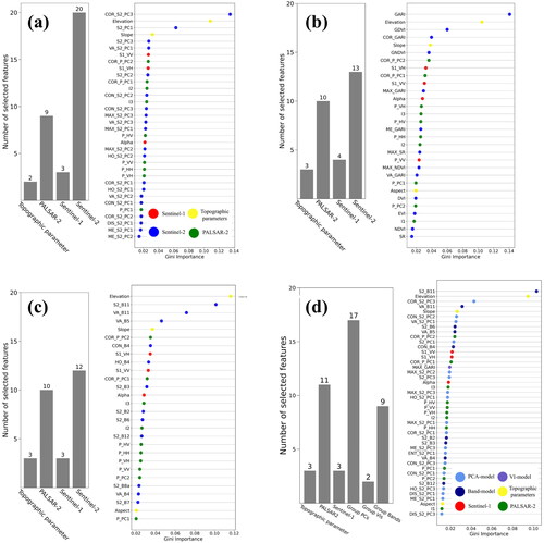
Figure 9. (a) Estimated wall-to-wall AGB of DBF in Oita prefecture, Japan. (b) Comparison of total DBF aboveground biomass (AGB) between statistical data in the Japanese forest register and the satellite-based model in city level. (c) First group. (d) Second group. Each data point represents the cumulative AGB at each of 18 cities (villages, towns, and cities) in Oita prefecture. $y^{\frac{1}{4}}\mathrm{x}$ is masked in red dotted line. 95% Confidence Interval is drawn in blue area.

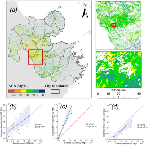
Figure 10. Correlation coefficient matrix between selected features: (a) PCA-model (b) VI-model, (c) Band-model, and (d) All data.

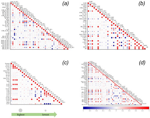
Table 3. Variance inflation factor in each group.

RF-based model	VIF
PCA-model	1126
VI-model	13247214379
Band-model	14191201649
All data	8832761381

Figure 11. Correlations between individual input bands and output component, (a) PC1 78.2% of dataset variance; (b) PC2 19.4% of dataset variance; (c) PC3, 1.33% of dataset variance; (d) Summarize of PCA proportion.

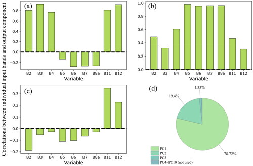
Table Appendix 1. Vegetation indices calculated from Sentinel-2 and PALSAR-2 used in this study.

Source	Indices	Equations
S2
	NDVI	$\frac{(\mathit{NIR}-\mathit{Re}d)}{(\mathit{NIR}+\mathit{Re}d)}$
	EVI	$\frac{2.5\mathrm{*}(\mathit{NIR}-\mathit{Re}d)}{(\mathit{NIR}+6\mathrm{*}\mathit{Re}d-7.5\mathrm{*}\mathit{Blue}+1)}$
	GARI	$\frac{\mathit{NIR}-[\mathit{Green}-1.7\mathrm{*}(\mathit{Blue}-\mathit{Re}d)]}{\mathit{NIR}+[\mathit{Green}-1.7\mathrm{*}(\mathit{Blue}-\mathit{Re}d)]}$
	GDVI	$\mathit{NIR}-\mathit{Green}$
	GNDVI	$\frac{(\mathit{NIR}-\mathit{Green})}{(\mathit{NIR}+\mathit{Green})}$
	GRVI	$\frac{\mathit{NIR}}{\mathit{Green}}$
	SAVI	$\frac{1.5\mathrm{*}(\mathit{NIR}-\mathit{Re}d)}{(\mathit{NIR}+\mathit{Re}d+0.5)}$
	SR	$\frac{\mathit{NIR}}{\mathit{Re}d}$
	DVI	$\mathit{NIR}-\mathit{Re}d$
PALSAR-2
	I1	$HH-\mathrm{HV}$
	I2	$HH+\mathrm{HV}$
	I3	$(HV-HH)/(HH+\mathrm{HV})$

Rouse J, Haas RH, Schell JA, Deering DW. 1974. Monitoring vegetation systems in the Great Plains with ERTS. NASA Special Publication. 351(1974):309.

 Google Scholar

Huete A, Didan K, Miura T, Rodriguez EP, Gao X, Ferreira LG. 2002. Overview of the radiometric and biophysical performance of the MODIS vegetation indices. Remote Sens Environ. 83(1-2):195–213.

 Web of Science ®Google Scholar

Gitelson AA, Kaufman YJ, Merzlyak MN. 1996. Use of a green channel in remote sensing of global vegetation from EOS-MODIS. Remote Sens Environ. 58(3):289–298.

 Web of Science ®Google Scholar

Gitelson AA, Gritz Y, Merzlyak MN. 2003. Relationships between leaf chlorophyll content and spectral reflectance and algorithms for non-destructive chlorophyll assessment in higher plant leaves. J Plant Physiol. 160(3):271–282.

 PubMed Web of Science ®Google Scholar

Sripada RP. 2005. Determining in-season nitrogen requirements for corn using aerial color-infrared photography. North Carolina State University.

 Google Scholar

Gitelson AA, Merzlyak MN. 1998. Remote sensing of chlorophyll concentration in higher plant leaves. Adv Space Res. 22(5):689–692.

 Web of Science ®Google Scholar

Sripada RP, Heiniger RW, White JG, Meijer AD. 2006. Aerial color infrared photography for determining early in‐season nitrogen requirements in corn. Agronomy J. 98(4):968–977.

 Web of Science ®Google Scholar

Huete AR. 1988. A soil-adjusted vegetation index (SAVI). Remote Sens Environ. 25(3):295–309.

 Web of Science ®Google Scholar

Birth GS, McVey GR. 1968. Measuring the color of growing turf with a reflectance spectrophotometer 1. Agronomy J. 60(6):640–643.

 Web of Science ®Google Scholar

Tucker CJ. 1979. Red and photographic infrared linear combinations for monitoring vegetation. Remote Sens Environ. 8(2):127–150.

 Web of Science ®Google Scholar

Kim Y, Jackson T, Bindlish R, Lee H, Hong S. 2011. Radar vegetation index for estimating the vegetation water content of rice and soybean. IEEE Geosci Remote Sens Lett. 9(4):564–568.

 Web of Science ®Google Scholar

Huggannavar V, Shetty A. 2020. Biomass estimation using synergy of ALOS-PALSAR and landsat data in tropical forests of Brazil. Applications of Geomatics in Civil Engineering. Singapore: Springer; p. 593–603.

 Google Scholar