Urban surface water bodies mapping using the automatic k-means based approach and sentinel-2 imagery

Figures & data

Figure 1. (a) Geographic location of the study areas; (b) satellite image of the Zagreb, Croatia study area (SA1); (c) satellite image of the New Delhi, India study area (SA2); (d) satellite image of the Bhopal, Madhya Pradesh, India study area (SA3). All satellite images use the Sentinel-2 ‘true color’ composite (4–3–2).

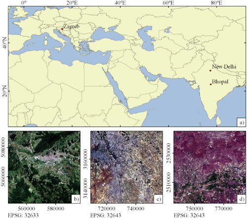
Table 1. Description of Sentinel-2 satellite imagery used in this research.

Study area	Sensing date	Satellite imagery ID
Zagreb, Croatia	27-July-2019	S2A_MSIL2A_20190627T095031_N0212_R079_T33TWL_20190627T142308
New Delhi, India	09-July-2019	S2A_MSIL2A_20190609T052651_N0212_R105_T43RGM_20190609T091600
Bhopal, India	27-May-2019	S2A_MSIL2A_20190527T051651_N0212_R062_T43QGF_20190527T093017

Figure 2. Statistical parameters for the accuracy assessments of the four variations in the AUWM calculated based on various numbers of k-means classes for SA1.

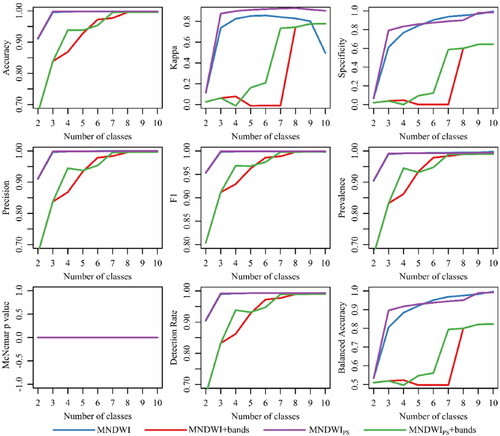
Figure 3. Statistical parameters for the accuracy assessment of the four variations in the AUWM calculated based on the various numbers of k-means classes for SA2.

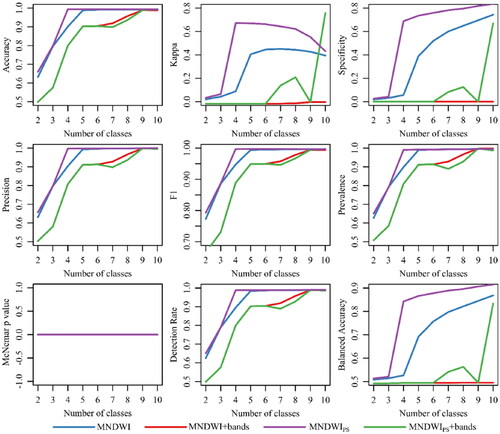
Figure 4. Statistical parameters for the accuracy assessment of the four variations in the AUWM calculated based on the various numbers of k-means classes for SA3.

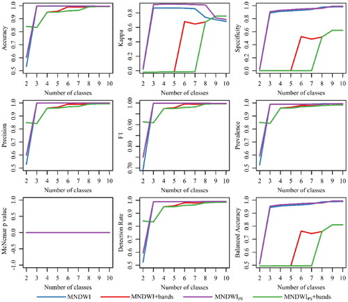
Figure 5. Processing time of the four variations in the AUWM, calculated based on the various numbers of k-means classes for (a) SA1, (b) SA2, (c) SA3, and (d) the average processing time of all three study areas.

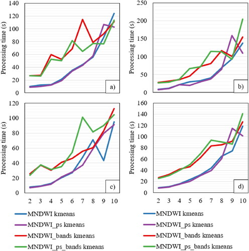
Table 2. Comparison of the statistical parameters and processing times for the MNDWI_PS calculated based on the various numbers of k-means classes. Bolded values represent lowest processing time MNDWI_PS with highest statistical parameters. Gray shaded column represents optimal number of classes for k-means for the MNDWI_PS.

k-means classes no.	2	3	4	5	6	7	8	9	10
Time(s)	8.05	9.94	15.07	20.14	30.58	39.36	60.42	114.81	101.23
Accuracy	0.73	0.93	1.00	1.00	1.00	1.00	1.00	1.00	1.00
Kappa	0.06	0.62	0.83	0.83	0.83	0.83	0.82	0.73	0.68
Specificity	0.04	0.58	0.82	0.84	0.86	0.88	0.89	0.93	0.94
Precision	0.72	0.93	1.00	1.00	1.00	1.00	1.00	1.00	1.00
F1	0.83	0.96	1.00	1.00	1.00	1.00	1.00	1.00	1.00
Prevalence	0.72	0.92	0.99	0.99	0.99	0.99	0.99	0.99	1.00
McNemar p value	0.00	0.00	0.00	0.00	0.00	0.00	0.00	0.00	0.00
Detection Rate	0.72	0.92	0.99	0.99	0.99	0.99	0.99	0.99	0.99
Balanced Accuracy	0.52	0.79	0.91	0.92	0.93	0.94	0.94	0.96	0.97

Figure 6. Statistical parameters for the accuracy assessment of the GSWD and AUWM calculated for all study areas.

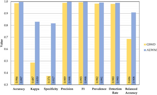
Figure 7. Visual comparison of the GSWD and AUWM for all study areas.

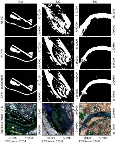
Figure 8. Surface water map for Croatia made using the AUWM. The enlarged subset (right) shows the area of Karlovac, known as the city situated on four rivers. Sentinel-2 ‘true color’ composite (4–3–2) was used for the comparison.

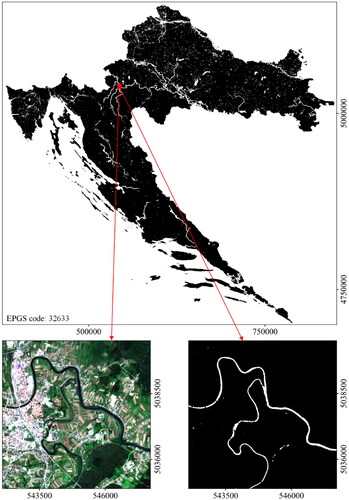
Figure A1. Visual analyses of the four variations in the AUWM, calculated based on the various numbers of k-means classes (2, 3, 5, and 10) for SA1.

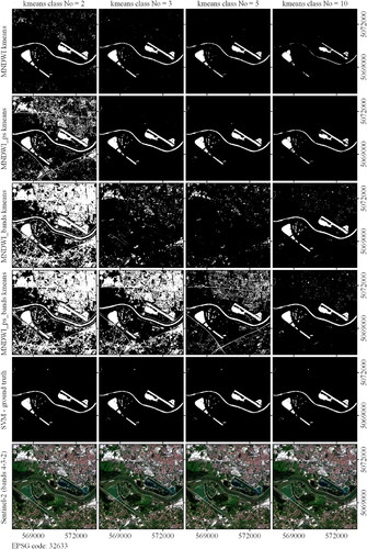
Figure A2. Visual analyses of the four variations in the AUWM, calculated based on the various numbers of k-means classes (2, 3, 5, and 10) for SA2.

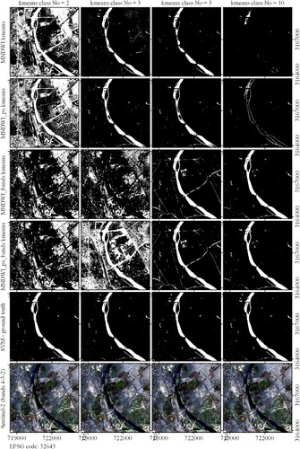
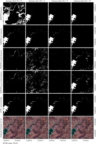
Figure A3. Visual analyses of the four variations in the AUWM, calculated based on the various numbers of k-means classes (2, 3, 5, and 10) for SA3.