Optimization design of quality monitoring network of Urmia plain using genetic algorithm and vulnerability map

Figures & data

Figure 1. General location of the study area with geological map and spatial distribution of EC values.

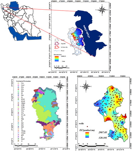
Figure 2. Geological section map of Urmia plain aquifer.

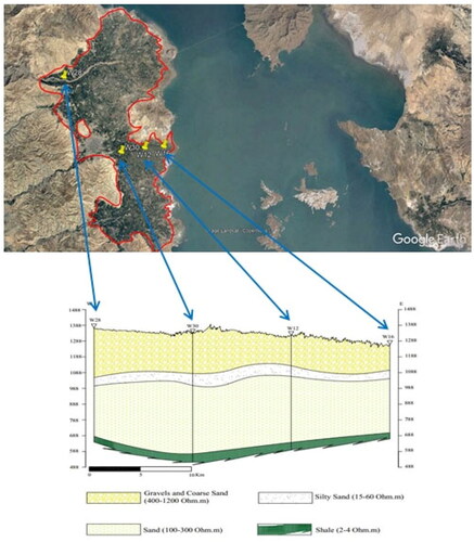
Figure 3. (a) Type of aquifer; (b) Hydraulic conductivity map; (c) Level difference map of underground water with sea level; (d) Distance map from the shoreline; (e) Developing map of seawater intrusion; (f) Aquifer thickness map; (g) Hydraulic gradient map, (h): Pumping rate map.

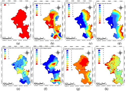
Table 1. Weights and ratings of the GALDIT and GALDIT-iP parameters (Chachadi 2005; Docheshmeh Gorgij and Asghari Moghaddam 2015).

Aquifer type		Hydraulic conductivity (m/day)		Height of groundwater level of above sea level (m)		Distance from the shoreline (m)
Weight = 1		Weight = 2		Weight = 5		Weight = 3
Range	Rate	Range	Rate	Range	Rate	Range	Rate
Free	9	<1.5	1	8.6–12	10	<1000	10
		1.5–2.5	3	12–17	8	1000–2000	9
		2.5–3.5	5	17–22	6	2000–3000	8
		3.5–6	8	22–27	5	3000–4000	7
		6–10	9	27–32	3	4000–5000	6
		>10	10	32–37	2	5000–6000	5
				37	1	6000–8000	3
						8000–10000	3
						10000-15000	2
						>15000	1
Impact of existing status of seawater intrusion in the area (mEq/L)		Aquifer thickness(m)		Hydraulic gradient		Pumping rates (m^3 per year)
Weight = 6		Weight = 3		Weight = 4		Weight = 4
Range	Rate	Range	Rate	Range	Rate	Range	Rate
<0.1	1	<80	1	<0.003	10	<2000	3
0.1–0.2	3	80–100	3	0.003–0.005	9	2000–5000	5
0.2–0.3	5	100–125	5	0.005–0.007	8	5000–10000	6
0.3–0.5	7	125–150	6	0.007–0.009	7	10000–25000	7
0.5–1	9	150–175	7	0.009–0.01	6	25000–50000	8
>1	10	175–200	8	0.01–0.05	5	50000–100000	9
		200–220	9	0.05–0.1	4	>100000	10
		>220	10	0.1–0.12	3
				0.12–0.14	2
				>0.14	1

Figure 4. Overview process of the GA.

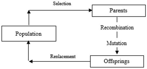
Figure 5. The vulnerability map of coastal aquifer of Urmia plain using modified GALDIT-iP.

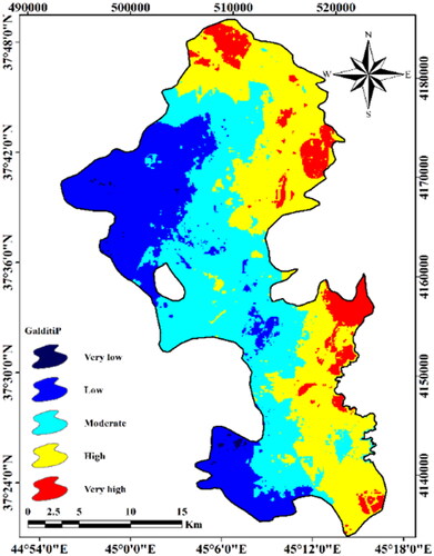
Table 2. Classification and percentages of vulnerable areas obtained from GALDIT-iP index.

Area (%)	Area (km^2)	Range	Classification
0.02	1.53	3–3.75	Very low
23.80	178.09	3.75–4.5	Low
35.21	263.48	4.5–5.25	Moderate
33.67	251.97	5.25–6	High
7.12	53.32	6–8	Very high
100	748.39	Sum

Table 3. Results obtained for different w values.

Weighting coefficient (w)	Correlation between EC and vulnerability (Z1)	Ratio between the number of all available monitoring wells and selected wells (Z2)	NS model efficiency (Z3)	Objective function (Zn)	Number of selected wells (n)
0.01	0.952	0.316	0.978	1.927	234
0.1	0.942	0.270	0.9841	1.899	200
0.2	0.950	0.240	0.9843	1.887	178
0.3	0.951	0.206	0.978	1.867	153
0.4	0.948	0.182	0.974	1.849	135
0.5	0.938	0.188	0.966	1.810	139
0.6	0.939	0.167	0.971	1.810	124
0.7	0.940	0.135	0.979	1.824	100
0.8	0.942	0.126	0.980	1.822	93
0.9	0.918	0.142	0.971	1.762	105
1	0.935	0.123	0.979	1.791	91
10	0.792	0.113	0.964	0.622	84
100	0.621	0.074	0.894	−5.907	55
1000	0.650	0.101	0.948	−99.617	75

Figure 6. Interpolation map of EC matching for (a) w = 1 and (b) w = 10 and vulnerability map matching for (c) w = 1 and (d) w = 10.

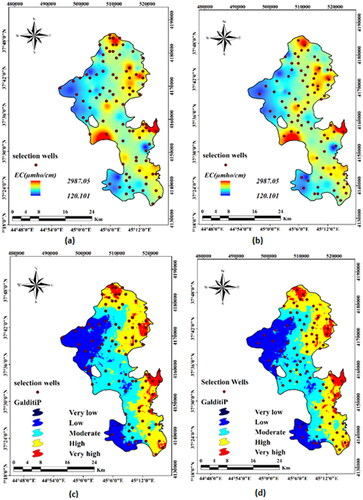
Figure 7. Validation of correlation coefficient of optimal wells for different w values.

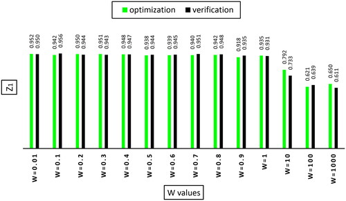
Figure 8. Validation of Nash-Sutcliffe coefficient model of optimal wells for different w values.

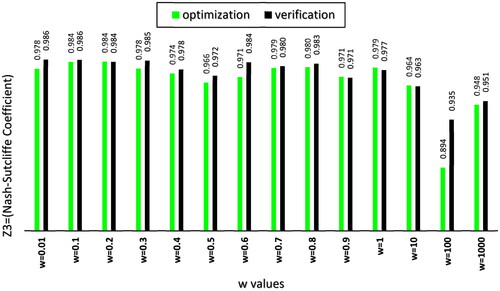
Table 4. Validation outcomes for different weights w values.

Weighting coefficient (w)	Optimization (95)				Verification (97)
	PBIAS	RMSE	S	r	PBIAS	RMSE	S	r
0.01	0.321	57.135	372.436	0.952	0.264	38.817	319.889	0.950
0.1	−0.157	47.247	361.662	0.942	−0.311	42.477	348.019	0.956
0.2	−0.245	48.720	380.588	0.950	−0.147	44.996	347.443	0.944
0.3	0.081	58.549	383.133	0.951	0.111	42.915	345.195	0.943
0.4	0.591	60.960	355.856	0.948	0.444	54.813	349.155	0.947
0.5	1.434	78.075	386.651	0.938	1.222	67.673	376.868	0.944
0.6	0.010	69.783	378.327	0.939	0.051	47.316	357.660	0.945
0.7	1.081	60.781	400.752	0.940	1.051	52.351	356.711	0.951
0.8	−0.453	62.094	415.268	0.942	−0.110	47.886	353.136	0.948
0.9	1.345	76.572	419.738	0.918	1.348	70.837	371.356	0.935
1	1.073	77.892	350.813	0.935	0.851	54.369	335.073	0.931
10	−0.892	56.885	282.989	0.792	−0.756	58.791	285.260	0.733
100	−1.044	103.770	282.988	0.621	−1.093	78.328	285.644	0.639
1000	0.979	80.598	327.554	0.650	0.911	68.216	267.619	0.611

Table 5. The change of mean EC values in monitored groundwater quality (unit: µSiemens/cm).

Year:1395	Without optimization	With optimization
W	–	0.01	0.1	0.5	1	10	100	1000
n	n = 109	234	200	139	91	84	55	75
Mean EC	929.633	865.872	867.205	876.418	1043.830	901.631	909.580	937.400

Chachadi AG. 2005. Seawater intrusion mapping using modified GALDIT indicator model-case study in Goa. Jalvigyan Sameeksha. 20:29–45.

 Google Scholar

Docheshmeh Gorgij A, Asghari Moghaddam A. 2015. Vulnerability assessment of saltwater intrusion using simplified GAPDIT Method: a case study of Azarshahr Plain Aquifer, East Azerbaijan, Iran.

 Google Scholar