Estimating forest aboveground biomass using temporal features extracted from multiple satellite data products and ensemble machine learning algorithm

Figures & data

Figure 1. The forest types and forest AGB data across California; the dot points correspond to forest AGB at a 500 m spatial resolution obtained by aggregating the lidar-derived biomass at a 30 m spatial resolution.

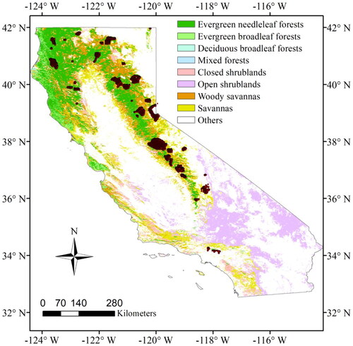
Table 1. The data sets of the MODIS data products used for AGB estimation.

Product	Layers	Spatial resolution	Temporal resolution	Reference
MOD09A1	Surface reflectance bands 1–7	500 m	8 days	Vermote et al. (1997; 2002)
MCD15A2	LAI and FAPAR	500 m	8 days	Myneni et al. (2002; 2015)
MOD17A2	GPP	500 m	8 days	Running et al. (2015) and Zhao et al. (2005)

Table 2. The temporal features used for modeling AGB under 18 scenarios.

Scenarios	Name	Layers used
Individual layer	Band 1	MODIS SR band 1
	Band 2	MODIS SR band 2
	Band 3	MODIS SR band 3
	Band 4	MODIS SR band 4
	Band 5	MODIS SR band 5
	Band 6	MODIS SR band 6
	Band 7	MODIS SR band 7
	LAI	MODIS LAI
	FAPAR	MODIS FAPAR
	GPP	MODIS GPP
Combination of layers	LAI–CH	MODIS LAI and CH
	FAPAR–CH	MODIS FAPAR and CH
	GPP–CH	MODIS GPP and CH
	SR	MODIS SR bands 1, 4, and 6
	SR–CH	MODIS SR bands 1, 4, and 6 and CH
	LFG	MODIS LAI, FAPAR, and GPP
	LFG–CH	MODIS LAI, FAPAR, GPP, and CH
	All	MODIS SR bands 1, 4, and 6; LAI; FAPAR; GPP; and CH

Figure 2. The accuracy of forest AGB estimated using the annual time-series data under the 18 scenarios; (a), (b), and (c) respectively represent the average R², RMSE, and bias values achieved by the AGB models developed under the 18 scenarios listed in Table 2.

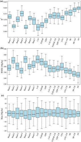
Figure 3. The accuracy of forest AGB estimated using the seasonal time-series data under the 10 scenarios; (a), (b), and (c) respectively represent the seasonal R², RMSE, and bias values achieved by the AGB models developed under the 18 scenarios; the error bars show the 95% confidence intervals.

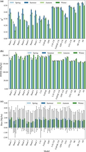
Figure 4. The accuracy of the forest AGB estimated using the temporal features selected by the AAF, SCC, PCP, and SAP methods; (a), (b), and (c) respectively represent R², RMSE, and bias values achieved under the 18 scenarios; the error bars show the 95% confidence intervals.

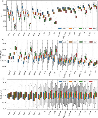
Figure 5. The density scatter plots of the reference AGB versus the AGB estimated by the AAF, SCC, PCP, and SAP methods and the five-fold cross-validation.

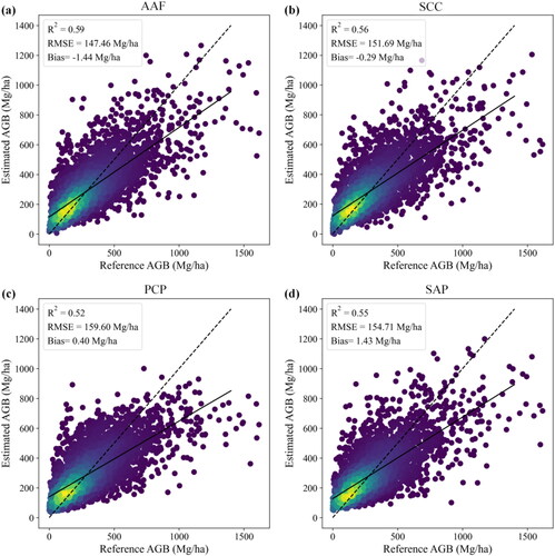
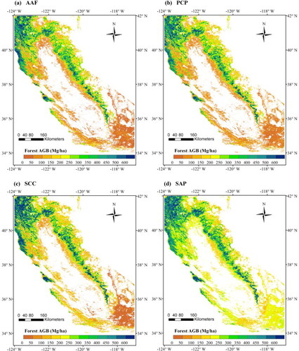
Figure 6. The spatial distribution of the forest AGB in 2013 estimated by the AAF, SCC, PCP, and SAP methods and the XGBoost algorithm based on the SR–CH data.

Data availability

The data that support the findings of this study are available on request from the corresponding author.