Comparison of a Sentinel-2 land cover map obtained through multi-temporal analysis with the official forest cartography. the case of Galicia (Spain)

Figures & data

Figure 1. Study area.

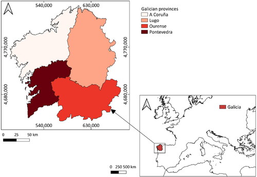
Table 1. Satellite images downloaded.

TMH	TNH	TPJ	TPH	TPG	TNG	TNJ
20190103	20190108	20190105	20190105	20190105	20190110	20190105
20190212	20190212	20190214	20190224	20190224	20190214	20190212
20190329	20190329	20190326	20190311	20190316	20190321	20190324
20190503	20190428	20190420	20190430	20190420	20190430	20190428
20190513	20190513	20190530	20190530	20190505	20190505	20190513
20190528	20190528	20190719	20190629	20190629	20190530	20190712
20190722	20190712	20190724	20190719	20190719	20190719	20190724
20190821	20190816	20190823	20190803	20190803	20190813	20190816
20190915	20190915	20190912	20190912	20190907	20190912	20190915
20191010	20191010	20191007	20191007	20191007	20191007	20191010
20191204	20191204	20191121	20191226	20191022	20191022	20191129
20191229	20191229	20191226		20191231	20191229	20191204

First column indicates Sentinel-2 tile. Next column indicates the date.

Figure 2. Detail of an MFE polygon and the corresponding attribute tables. Reference image: 2017 PNOA image (MTMAU 2022).

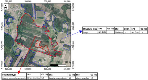
Figure 3. Distribution of the training polygons.

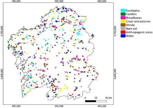
Figure 4. Distribution of the verification points.

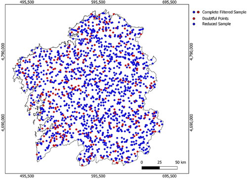
Figure 5. Example of the MFE attribute table after harmonization. Reference image: 2017 PNOA image (MTMAU 2022).

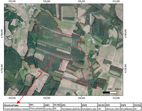
Table 2. Equivalences between the MFE tree species and the LCMG19 land cover classes.

Code of harmonized class	LCMG19 class	MFE species
1	Eucalyptus	Eucalyptus spp.
2	Conifers	Cedrus spp.
		Chamaecyparis spp.
		Cupressus spp.
		Other conifers
		Picea spp.
		Pinus spp.
		Pseudotsuga spp.
		Taxus spp.
		Thuja spp.
3	Broadleaves	Acacia spp.
		Acer spp.
		Ailanthus spp
		Alnus spp
		Arbutus spp.
		Betula spp.
		Castanea spp.
		Corylus spp.
		Crataegus spp.
		Fagus spp.
		Fraxinus spp.
		Ilex spp.
		Juglans spp.
		Laurus spp.
		Pistacia spp.
		Platanus spp.
		Populus spp.
		Prunus spp.
		Pyrus spp.
		Quercus spp.
		Robinia spp.
		Salix spp.
		Sorbus spp.
		Ulmus spp.

Figure 6. Diagram of the procedure followed to compare the Spanish forest official cartography (the MFE) and the land cover map of Galicia produced using Sentinel-2 processing (the LCMG19). ESP1: the MFE raster layer containing the primary species (SP1) information, after legend harmonization. ESP2: the MFE raster layer containing the secondary species (SP2) information, after legend harmonization. ESP3: the MFE raster layer containing the tertiary species (SP3) information, after legend harmonization.

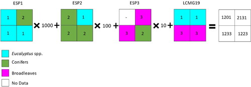
Figure 7. Spatial comparison of the LCMG19 and the MFE. Examples of Level 1, Level 2, and Level 3 matches.

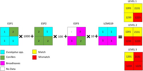
Figure 8. Land cover map of Galicia 2019 (LCMG19).

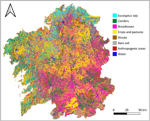
Table 3. Confusion matrix obtained from the cross verification of the LCMG19 using the complete filtered sample.

Reference/ Classified	1	2	3	4	5	6	7	8	T	UA (%)
1	138	15	0	0	0	0	0	0	153	90
2	20	199	12	2	15	0	0	1	249	80
3	24	13	286	13	52	1	0	0	389	74
4	8	2	17	406	40	6	8	0	487	83
5	9	13	6	7	195	1	2	0	233	84
6	1	3	0	5	14	49	14	0	86	57
7	0	0	0	2	2	9	34	0	47	72
8	0	0	0	0	0	0	0	12	12	100
T	200	245	321	435	318	66	58	13	1656	OA (%)
PA (%)	69	81	89	93	61	74	59	92	OA (%)	80
F1 score	0.78	0.81	0.81	0.88	0.71	0.64	0.65	0.96	KI	0.75

Classes: Eucalyptus spp. (1), Conifers (2), Broadleaves (3), Crops and pastures (4), Shrubs (5), Bare soil (6), Anthropogenic areas (7) and Water (8). Metrics: User’s Accuracy (UA), Producer’s Accuracy (PA), Overall Accuracy (OA), T: Total, KI: Kappa Index.

Table 4. Confusion matrix obtained from the cross verification of the LCMG19 using the reduced sample.

Reference/ Classified	1	2	3	4	5	6	7	8	T	UA (%)
1	104	11	0	0	0	0	0	0	115	90
2	10	167	5	1	7	0	0	1	191	87
3	8	2	257	9	30	0	0	0	306	84
4	5	1	13	371	21	1	7	0	419	89
5	5	8	2	4	164	0	2	0	185	89
6	0	0	0	2	11	29	13	0	55	53
7	0	0	0	2	2	4	32	0	40	80
8	0	0	0	0	0	0	0	11	11	100
T	132	189	277	389	235	34	54	12	1322	OA (%)
PA (%)	79	88	93	95	70	85	59	92	OA (%)	86
F1 score	0.84	0.88	0.88	0.92	0.78	0.65	0.68	0.96	KI	0.82

Classes: Eucalyptus spp. (1), Conifers (2), Broadleaves (3), Crops and pastures (4), Shrubs (5), Bare soil (6), Anthropogenic areas (7) and Water (8). Metrics: User’s Accuracy (UA), Producer’s Accuracy (PA), Overall Accuracy (OA), T: Total, KI: Kappa Index.

Table 5. Comparison of the LCMG19 and the MFE in terms of the surface area covered by the tree-related classes (in hectares).

Class	A Coruña (ha)	Lugo (ha)	Ourense (ha)	Pontevedra (ha)	Galicia (ha)
Eucalyptus	−48.455	−7.899	1.104	−21.827	−77.078
Conifers	−33.858	−55.043	−39.696	−24.594	−153.190
Broadleaves	86.566	88.984	41.591	48.921	266.062

Results are provided per province and for the whole region of Galicia.

Table 6. Comparison of the LCMG19 and the MFE in terms of the surface area covered by the tree-related classes (in percentage).

Class	A Coruña	Lugo	Ourense	Pontevedra	Galicia
Eucalyptus	−27%	−12%	88%	−35%	−25%
Conifers	−24%	−32%	−36%	−29%	−30%
Broadleaves	134%	44%	25%	109%	56%

Results are provided per province and for the whole region of Galicia.

Figure 9. Graphical representation of the spatial comparison of the Eucalyptus spp. distribution in the LCMG19 and the MFE Level 1: the LCMG19 vs the MFE considering SP1, SP2 and SP3. In green: pixel matches; in red: pixel mismatches.

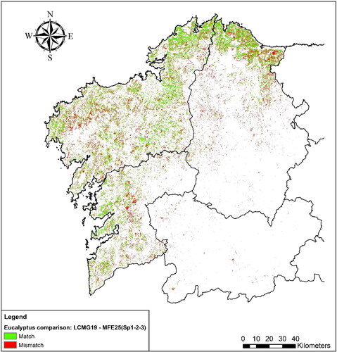
Figure 10. Graphical representation of the spatial comparison of the Eucalyptus spp. distribution in the LCMG19 and the MFE Level 2: the LCMG19 vs the MFE considering SP1 and SP2. In green: pixel matches; in red: pixel mismatches.

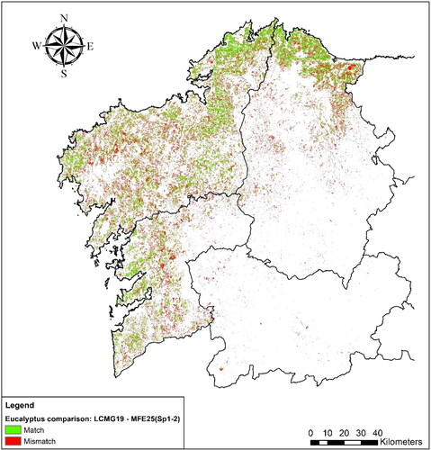
Figure 11. Graphical representation of the spatial comparison of the Eucalyptus spp. distribution in the LCMG19 and the MFE Level 3: the LCMG19 vs the MFE considering only SP1. In green: pixel matches; in red: pixel mismatches.

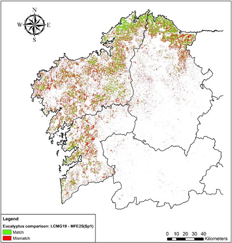
Figure 12. Graphical representation of the spatial comparison of the Conifers distribution in the LCMG19 and the MFE Level 1: the LCMG19 vs the MFE considering SP1, SP2 and SP3. In green: pixel matches; in red: pixel mismatches.

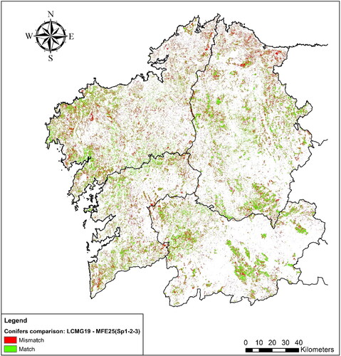
Figure 13. Graphical representation of the spatial comparison of the Conifers distribution in the LCMG19 and the MFE Level 2: the LCMG19 vs the MFE considering SP1 and SP2. In green: pixel matches; in red: pixel mismatches.

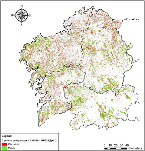
Figure 14. Graphical representation of the spatial comparison of the Conifers distribution in the LCMG19 and the MFE Level 3: the LCMG19 vs the MFE considering only SP1. In green: pixel matches; in red: pixel mismatches.

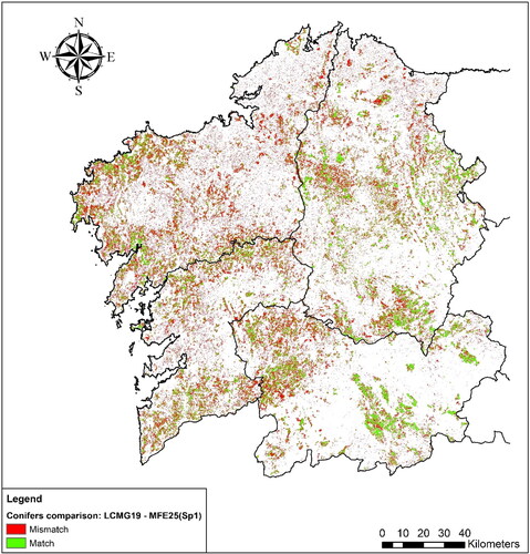
Figure 15. Graphical representation of the spatial comparison of the Broadleaves distribution in the LCMG19 and the MFE Level 1: the LCMG19 vs the MFE considering SP1, SP2 and SP3. In green: pixel matches; in red: pixel mismatches.

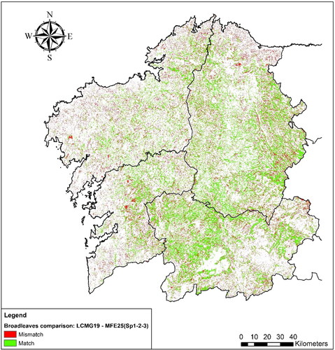
Figure 16. Graphical representation of the spatial comparison of the Broadleaves distribution in the LCMG19 and the MFE Level 2: the LCMG19 vs the MFE considering SP1 and SP2. In green: pixel matches; in red: pixel mismatches.

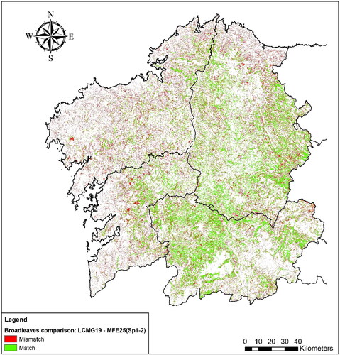
Figure 17. Graphical representation of the spatial comparison of the Broadleaves distribution in the LCMG19 and the MFE Level 3: the LCMG19 vs the MFE considering only SP1. In green: pixel matches; in red: pixel mismatches.

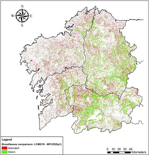
Figure 18. Graphical representation of the spatial agreement of tree classes in the LCMG19 and the MFE. Comparison of the LCMG19 and the MFE considering SP1, SP2 and SP3. In green: pixel matches; in red: pixel mismatches.

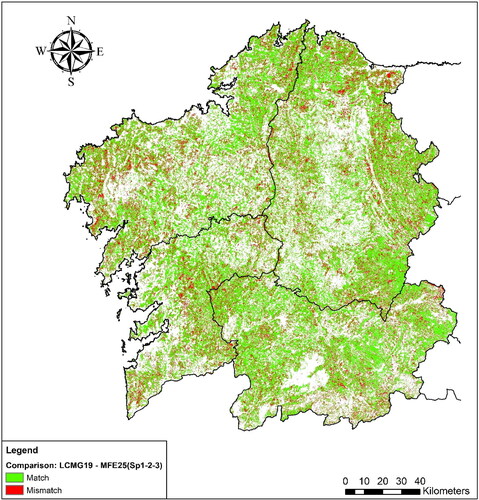
Figure 19. Graphical representation of the spatial agreement of tree classes in the LCMG19 and the MFE. Comparison of the LCMG19 and the MFE considering SP1 and SP2.In green: pixel matches; in red: pixel mismatches.

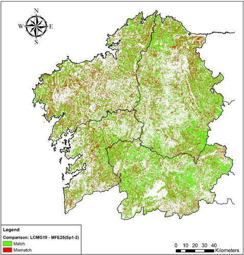
Figure 20. Graphical representation of the spatial agreement of tree classes in the LCMG19 and the MFE. Comparison of the LCMG19 and the MFE considering only SP1. In green: pixel matches; in red: pixel mismatches.

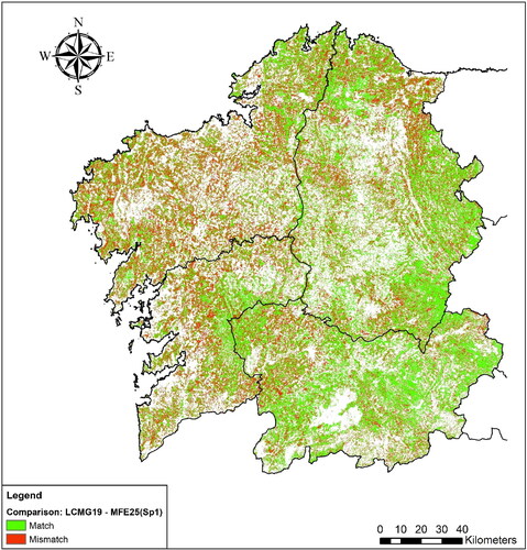
Table 7. Quantitative results of the spatial comparison of the MFE and the LCMG19: percentages of matching pixels.

Area	Reference	Estimated	Eucalyptus match (%)	Conifers match (%)	Broadleaves match (%)	Tree cover match (%)
Galicia	MFE	LCMG19	58	55	79	66
	LCMG19	MFE	80	76	65	70
A Coruña	MFE	LCMG19	59	60	86	66
	LCMG19	MFE	86	75	53	70
Lugo	MFE	LCMG19	56	56	80	68
	LCMG19	MFE	71	77	68	71
Ponte vedra	MFE	LCMG19	57	53	87	64
	LCMG19	MFE	81	74	59	69
Ourense	MFE	LCMG19	40	50	74	66
	LCMG19	MFE	13	79	70	72

Reference: The map that is considered to be the ground truth. Estimated: The map that is evaluated.

Figure 21. Comparison between the MFE (A) and the LCMG19 (B).

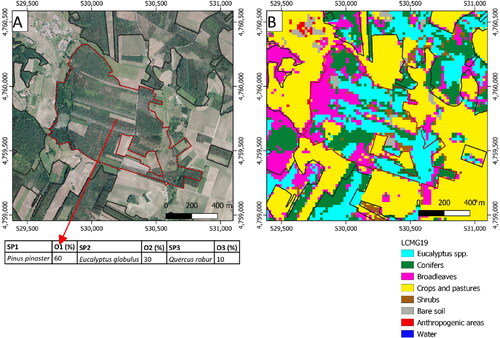
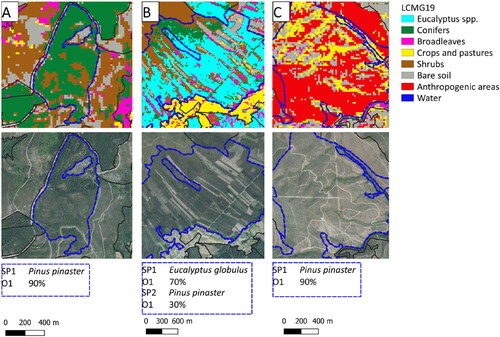
Figure 22. Examples of discrepancies between the MFE and the LCMG19.

Data availability statement

The data that support the findings of this study are available from the corresponding author, J.A, upon reasonable request.