Applicability of SWOT data in calibrating WRF-Hydro hydrological model over the Tawa River basin

Figures & data

Figure 1. Map of study area representing study domain, Hoshangabad gauge station location, SWOT calibration and validation orbital pass over the Narmada River.

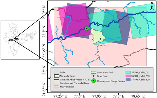
Table 1. WRF-Hydro calibration parameter, definition, and scaling factor ranges considered in calibration process.

Parameter	Definition	Range of parameter value	Reference parameter value	Calibrated parameter values
				for Qg	for Qgt	for Qs
REFKDT	Runoff infiltration	0.5-1.5	0.50	1.20	1.26	1.35
RETDEPRTFAC	Surface retention depth	0-10	1.00	4.50	3.29	3.20
OVROUGHRTFAC	Surface roughness	0.1-1	1.00	0.59	0.54	0.53
Manning’s roughness	Channel roughness	0.5-0.00125	0.40	0.03	0.03	0.02

Figure 2. Methodology flowchart for calibrating WRF-Hydro model using DDS algorithm.

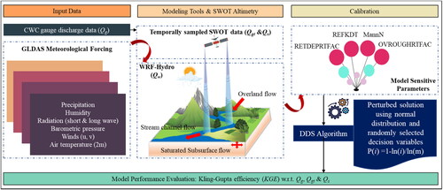
Figure 3. WRF-Hydro model calibration performance using KGE for different normalized parameter values obtained by the best iteration of the DDS algorithm targeting the different discharge: (a) Q_g, (b) Q_gt, and (c) Q_s. The x-axis represents the best model iteration, the left vertical axis represents the model performance by KGE, and the right vertical axis represents the normalized values of parameters selected by the DDS algorithm for calibrating the model. The normalized values of parameters have been shown to represent better parameter values having varied scales.

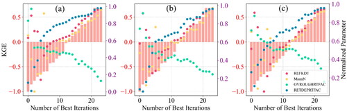
Figure 4. Calibration of discharge with optimized Model-A, Model-B, and Model-C parameters for the (a) Event -1, (b) Event-2, and (c) Event-3 at Hoshangabad gauge station.

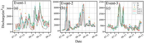
Figure 5. Density curve of the percentage difference between time series Q_g-Q_gt and Q_g-Q_s. The density curve having an area equal to one represents the effect of SWOT TS alone (Q_g-Q_gt) and when combined with the uncertainty associated (Q_g-Q_s) over the KGE values in each iteration. The outlier has not been shown.

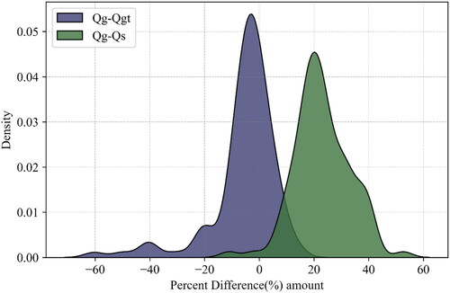
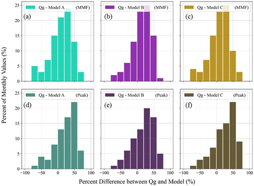
Figure 6. Histogram of the percentage difference between Q_g and monthly mean flow (MMF) i.e. (a) Qg-Model A, (b) Qg-Model B, (c) Qg-Model C and monthly peak flow i.e. (d) Qg-Model A, (e) Qg-Model B, (f) Qg-Model C for 2015-2017.