Integrated generalization method of contours and rivers considering geographic characteristics

Figures & data

Figure 1. Contours and rivers with a scale of 1:10,000 in the study area.

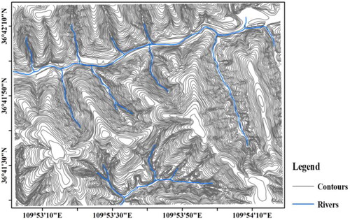
Table 1. Identification rules for parts of river network morphologies.

River network morphologies	Sinuosity	Intersection angle distribution ratio /%		Flow direction	Length
		acute angle	approximate square
Tree-like river network	<1.5	>70	<30	Tributaries join the mainstream at acute angles from different directions.	The length ratio does not change much, and the length of adjacent levels varies greatly.
Checkered river network	>1.5	<60	>40	There is a mutation in the flow direction.	The length ratio varies more with the length.
Feathery river network	<1.1	<30	>60	The direction of each branch is basically the same.	The length doesn’t change much.
Parallel river network	1.2–1.5	–	–	The mainstream is basical in the same direction, and the corresponding tributaries are also basical in the same direction.	The length ratio varies little with length.

Table 2. Classification of topographic feature lines.

Classification	Grade
Valley lines	Main valley line, first-level branch valley lines, second-level branch valley lines, and lower-branch valley lines
Ridge lines	Main ridge line, first-level branch ridge lines, and lower-level branch ridge lines
Saddle lines	–

Figure 2. Variation of the topological relationship between contours.

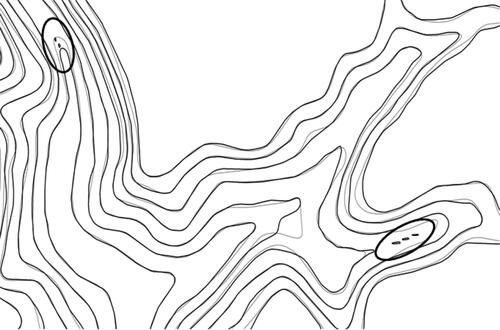
Figure 3. Gentle probability of topographic feature lines.

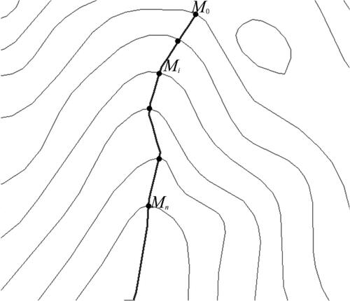
Figure 4. Spatial coupling between valley lines and less developed rivers. (a) Rivers with lower headwaters; (b) the area of the valley floor where rivers protrude but do not develop; (c) valley line headwaters are served as river headwaters; (d) the valley lines in the convex region of the valley floor ‘replace’ the rivers.

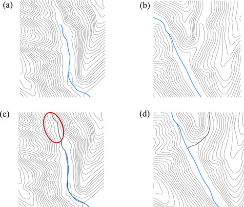
Figure 5. The positive intersection relationship between contours and rivers.

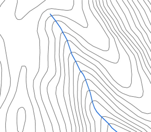
Figure 6. Diagram of point set rate segmentation.

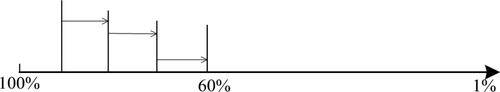
Figure 7. Flow chart of determining the reserved point rate for the target scale.

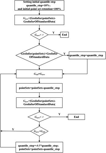
Figure 8. Bending division based on extreme points of line elements (Deng et al. 2013).

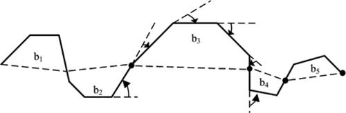
Figure 9. River network classification and the elevation change of river AB.

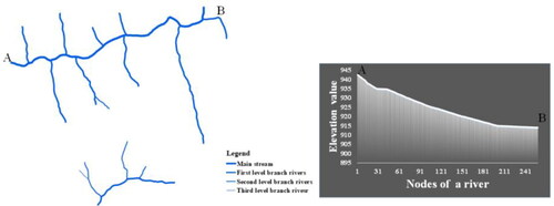
Table 3. Calculation results of river network parameters in the study area.

Study area	Whether there is a network loop	Sinuosity	Intersection angle distribution ratio /%
			Acute angle	The approximate square
Loess relief	null	1.08	28.6%	71.4%

Figure 10. Variation of river length ratio.

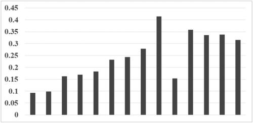
Figure 11. Extraction results of topographic feature lines.

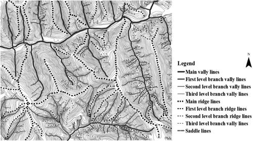
Figure 12. Spatial statistical characteristics of topographic feature lines.

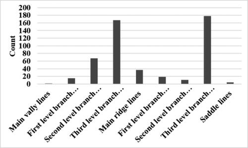
Table 4. Gentle probability distribution of topographic feature lines.

Different types of gentle probability distribution maps of topographic feature lines
Main-, first-, second-, and thrid-level branch valley lines	Main-, first-, second-, and thrid-level branch ridge lines

Table 5. Selection of topographic feature lines.

Topographic feature lines with gentle probability greater than 0	There are feature lines or local line segments that are spatially coupled with rivers	Saddle lines	The total number of selections
37	16	4	57

Table 6. Discretization information of each element.

Number of discrete points on contours	Number of discrete points on rivers	Number of discrete points on the selected topographic feature lines	The total number of discrete points
116,221	1205	1511	118,937

Table 7. Semantic information description and weighted for discrete points of different types.

Discrete points on contours			Discrete points on rivers
General discrete points	Special discrete points	The intersection points between contours and rivers	Mian rivers	First-level branch rivers	Second-level branch rivers	Third-level branch rivers	The intersection of rivers and contours, the first and last points of rivers, and the confluence points between rivers
1	1	+$\mathrm{\infty }$	10	8	6	4	+∞

Figure 13. Generalization results of loess relief. (a) Integrated generalization results with a scale of 1:25000; (b) integrated generalization results with a scale of 1:50,000.

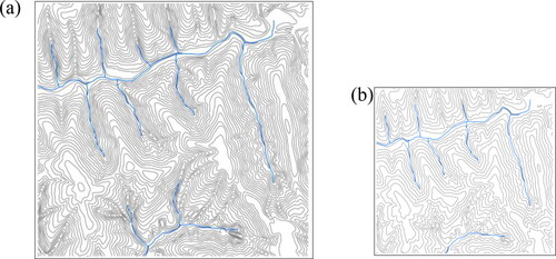
Table 8. Comparison of terrain accuracy information before and after loess relief generalization.

Scales	Average gradient	Maximum elevation	Minimum elevation	Average elevation	Standard deviation	Positive- and negative-terrain ratio
1:10000	31.49	1140	914.06	1018.98	50.24	1.04
1:25000	31.84	1140	914.06	1017.93	50.40	1.03
1:50000	31.82	1140	914.06	1014.672	51.06	1.06

Figure 14. Comparison of shadow maps at different scales in the study area. (a) Original shadow map with a scale of 1:10,000; (b) shadow map with a scale of 1:25,000; and (c) shadow map with a scale of 1:50,000.

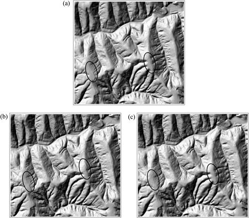
Table 9. Comparison of information volume before and after river reconstruction.

Scales	The bending geometric information content	The overall level shape maintenance information content
1:10,000	317.326	3.50354
1:25,000	314.382	3.50351
1:50,000	306.011	3.50323

Deng M, Fan ZD, Liu HM. 2013. Performance evaluation of line simplification algorithm based on hierarchical information content. Acta Geod et Cartogr Sin. 4-2(5):767–773,781. in Chinese)

 Google Scholar

Data availability statement

The dataset utilized/analyzed during the current study will be available from the corresponding author upon request.