Inversion of intertidal zone topography based on optimized random forest regression characteristic parameters

Figures & data

Figure 1. Step-by-step approach of intertidal zone topography inversion.

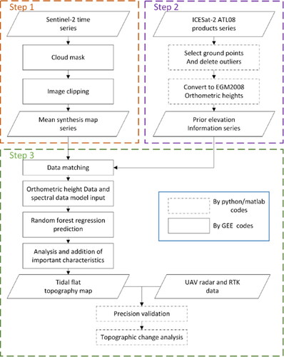
Table 1. Feature parameters for the model.

Feature name	Source or calculation formula
Band i (i = 1,…,12)	Sentinel 2 SR
Band 8 A	Sentinel 2 SR
SDD	$-5.838*\log \left(\frac{{\mathit{Band}}_4}{{\mathit{Band}}_1}\right)*\log \left(\frac{{\mathit{Band}}_4}{{\mathit{Band}}_2}\right)*\log \left(\frac{{\mathit{Band}}_3}{{\mathit{Band}}_4}\right)+1.101$
NDWI	$\frac{{\mathit{Band}}_3-{\mathit{Band}}_8}{{\mathit{Band}}_3+{\mathit{Band}}_8}$
SSC	$1.101*\frac{{\mathit{Band}}_4}{{\mathit{Band}}_3}+11.262*{\mathit{Band}}_8+0.76$
DATA_TP	$\frac{{\mathit{Data}}_{x1}}{{\mathit{Data}}_{x2}}$

Figure 2. Overview of the study area; (a) shows the general location of the study area, (b) and (c) are Sentinel-2 images on 18 February 2020 and 13 April 2020, respectively, the names of the areas in (b) and (c) are Sheyang estuary and Radiation Sandbar, respectively, which belong to the wider area of intertidal mudflats in Jiangsu, and the intertidal mudflats in Jiangsu north of Sheyang estuary are gradually decreasing in extent, the black dot pixels in (b) and (c) are schematic diagrams of some location points of ICESat-2 photon data in 2022 located in the intertidal mudflat area.

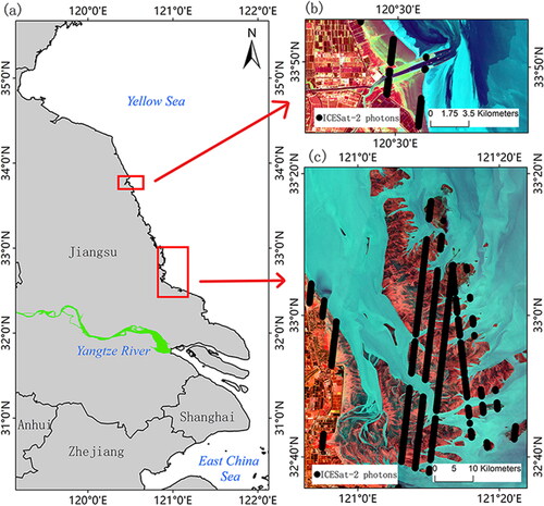
Figure 3. Sentinel-2 of T51SUS frame number image in 2020; image RGB band settings corresponding to band 8, band 3 and band 2 stretched display; time stamp in the upper right corner of each image is the imaging time.

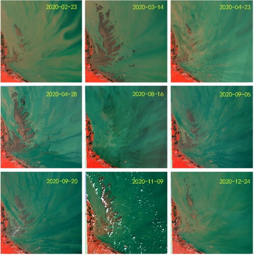
Table 2. Training results of different image set models.

Time (2020)	02/23-03/14	03/14	04/23	08/16	03/14-04/28	02/23-08/16	09/20-12/24	11/09	01/01-12/31
Number of images	2	1	1	1	3	5	3	1	9
MAE (m)	0.33	0.37	0.27	0.24	0.34	0.31	0.31	0.33	0.3
RMSE (m)	0.43	0.47	0.38	0.35	0.43	0.4	0.4	0.43	0.39
R^2	0.79	0.74	0.83	0.85	0.78	0.81	0.82	0.78	0.82

Figure 4. Correlation coefficient between predicted values from respective bands and observed value, Band1,…, Band12 represent Sentinel-2 multispectral bands, Obs is ICESat-2 photon orthometric heights.

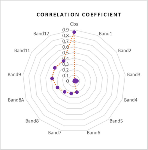
Figure 5. Feature importance ranking of model input parameters. Bandi_TP (i = 1,…,12,8 A) indicates the time-phase difference information for the band; the data has been normalized.

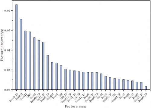
Figure 6. Validation of model predictions against ICESat-2 input data, with the color bar showing higher values for denser concentrations of points, and (a), (b), (c) and (d) representing the validation of intertidal topographic inversion predictions against ICESat-2 data for 2019, 2020, 2021 and 2022 respectively.

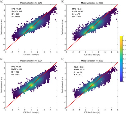
Figure 7. Estimated intertidal terrain accuracy assessment. (a) is a map of the inverse terrain and UAV LiDAR data verification; the calculated result is the difference between the UAV measured terrain and the inverted terrain, with a uniform spatial resolution of 10 m; (b) is a scatter diagram of the UAV data for validation, excluding the data from tidal trenches; (c) is a scatter diagram of verification of ICESat-2 data; (d) is a scatter diagram of RTK data for validation.

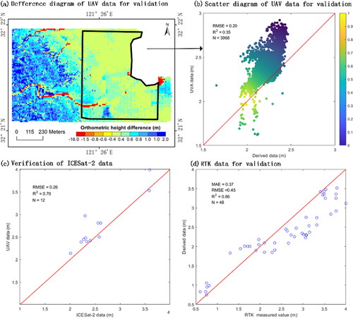
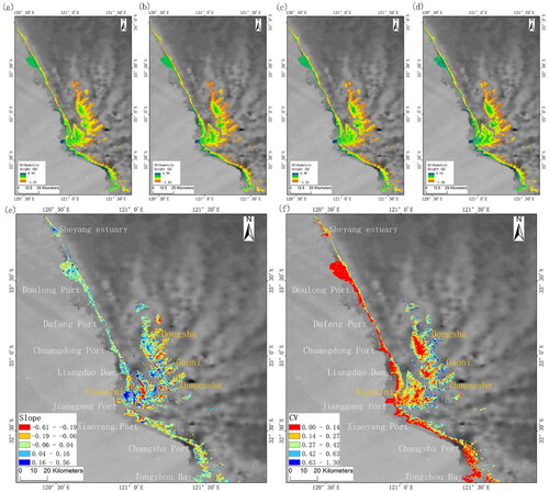
Figure 8. Intertidal topography inversion image. Figure 8(a–d) is the inverted intertidal topography in 2019, 2020, 2021 and 2022 with a spatial resolution of 10 m; Figure 8(e) is the slope of the topography in 2019–2022 with a spatial resolution of 500 m and Figure 8(f) is the variation coefficients of the topography in 2019–2022 with a spatial resolution of 500 m; the background of all images is from GEBCO data in 2022 (Group 2022).

Data availability statement

Data available on request from the authors.