Attention-based multiscale deep learning with unsampled pixel utilization for hyperspectral image classification

Figures & data

Figure 1. The workflow of the multiscale attention HybridSN integrated with UNet for HSI classification. The model combines the advantages of the multiscale attention HybridSN and the UNet to achieve improved performance in HSI classification.

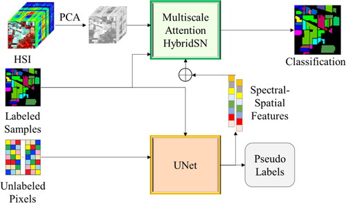
Figure 2. The workflow of the multiscale attention HybridSN model for HSI classification. The model is composed of three sets of 3D convolutional layers, each processing image patches of different scales (5x5, 7x7, and 11x11), and utilizing spectral attention before the 3D convolutional layers to weigh the importance of different spectral bands. The features learned from these 3D convolutional layers are then concatenated and passed through 2D convolutional layers, which employ spatial attention before the 2D convolutional layers to weigh the importance of different spatial locations. Finally, the output is obtained from a fully connected layer with the activation function of softmax.

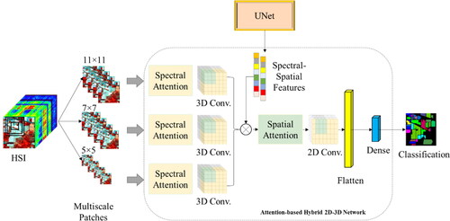
Figure 3. The UNet model architecture for HSI classification. This model consists of a series of 2D convolutional layers and up-sampling layers, with max pooling used to reduce the spatial dimensions. The architecture is symmetrical with a contracting path and an expanding path, which helps to preserve spatial information throughout the model. The final layer includes a dense layer and a softmax activation function to generate class probabilities.

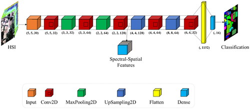
Figure 4. The architecture of spatial attention is used in this research. This component uses a combination of convolutional layers and pooling to learn and highlight the most informative spatial features in the input image.

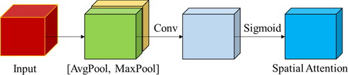
Figure 5. The spectral attention module in the multiscale attention HybridSN model for HSI classification. The module is designed to emphasize the important features in the spectral dimension and weigh them accordingly before the 3D convolutional layers process the input data.

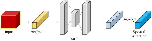
Table 1. The number of training, validation, and testing samples for the Indian Pines dataset.

Number	Name	Training	Validation	Testing	Total
1	Alfalfa	9	5	32	46
2	Corn-notill	286	142	1000	1428
3	Corn-min	166	83	581	830
4	Corn	47	24	166	237
5	Grass/Pasture	97	48	338	483
6	Grass/Trees	146	73	511	730
7	Grass/Pasture-mowed	6	3	19	28
8	Hay-windrowed	96	48	334	478
9	Oats	4	2	14	20
10	Soybean-notill	194	98	680	972
11	Soybean-mintill	491	246	1718	2455
12	Soybean-clean	119	59	415	593
13	Wheat	41	21	143	205
14	Woods	253	127	885	1265
15	Building-Grass-Trees-Drives	77	39	270	386
16	Stone-steel Towers	19	9	65	93
	Total	2051	1027	7171	10249

Table 2. The number of training, validation, and testing samples for the University of Pavia dataset.

Number	Name	Training	Validation	Testing	Total
1	Asphalt	1326	663	4642	6631
2	Meadows	3730	1865	13054	18649
3	Gravel	420	210	1469	2099
4	Trees	613	306	2145	3064
5	Metal sheets	269	135	941	1345
6	Bare soil	1006	503	3520	5029
7	Bitumen	266	133	931	1330
8	Bricks	736	368	2578	3682
9	Shadows	189	95	663	947
	Total	8555	4278	29943	42776

Table 3. The number of training, validation, and testing samples for the Houston University dataset.

Number	Name	Training	Validation	Testing	Total
1	Healthy Grass	247	124	865	1236
2	Stressed Grass	243	122	850	1215
3	Synthetic Grass	139	70	488	697
4	Tree	249	124	871	1244
5	Soil	248	124	870	1242
6	Water	65	33	227	325
7	Residential	251	126	878	1255
8	Commercial	249	124	871	1244
9	Road	245	123	857	1225
10	Highway	245	123	859	1227
11	Railway	244	122	852	1218
12	Parking Lot1	247	123	863	1233
13	Parking Lot2	94	47	328	469
14	Tennis Court	86	43	299	428
15	Running Track	132	66	462	660
	Total	2984	1494	10440	14918

Figure 6. OA (%) of the proposed model with different patch sizes in the three datasets.

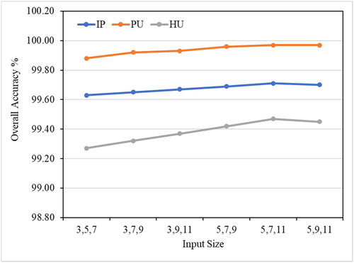
Figure 7. Classification maps of different models on the IP dataset. (a) Ground-truth map. (b) SVM. (c) 2D CNN. (d) 3D CNN. (e) HybridSN. (f) M3D-DCNN. (g) DBDA. (h) ACA-HybridSN. (i) MSA-HybridSN-U.

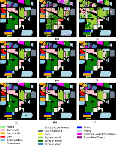
Figure 8. Classification maps of different models on the PU dataset. (a) Ground-truth map. (b) SVM. (c) 2D CNN. (d) 3D CNN. (e) HybridSN. (f) M3D-DCNN. (g) DBDA. (h) ACA-HybridSN. (i) MSA-HybridSN-U.

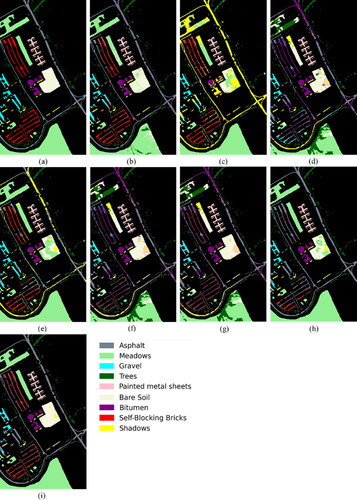
Figure 9. Classification maps of different models on the HU dataset. (a) Ground-truth map. (b) SVM. (c) 2D CNN. (d) 3D CNN. (e) HybridSN. (f) M3D-DCNN. (g) DBDA. (h) ACA-HybridSN. (i) MSA-HybridSN-U.

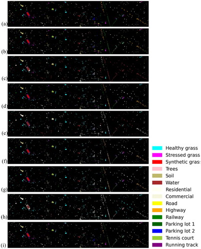
Table 4. Classification results of 5% samples of IP dataset.

Model	Classification Accuracy
	OA	AA	Kappa
SVM	74.77 ± 0.23	78.00 ± 0.09	0.710 ± 0.13
2D CNN	99.27 ± 0.03	99.42 ± 0.01	0.991 ± 0.02
3D CNN	99.72 ± 0.05	99.63 ± 0.02	0.996 ± 0.03
HybridSN	99.55 ± 0.02	99.53 ± 0.01	0.994 ± 0.01
M3D-DCNN	99.08 ± 0.05	99.03 ± 0.02	0.995 ± 0.03
DBDA	99.29 ± 0.06	99.51 ± 0.03	0.991 ± 0.04
ACA-HybridSN	99.66 ± 0.03	99.53 ± 0.01	0.996 ± 0.02
MSA-HybridSN-U	99.71 ± 0.01	99.65 ± 0.01	0.997 ± 0.02

Table 5. Classification results of 5% samples of PU dataset.

Model	Classification Accuracy
	OA	AA	Kappa
SVM	89.41 ± 0.30	91.14 ± 0.13	0.861 ± 0.16
2D CNN	99.96 ± 0.03	99.84 ± 0.01	0.999 ± 0.02
3D CNN	99.97 ± 0.02	99.83 ± 0.01	0.999 ± 0.02
HybridSN	99.79 ± 0.04	99.58 ± 0.02	0.997 ± 0.02
M3D-DCNN	99.24 ± 0.04	99.31 ± 0.02	0.996 ± 0.02
DBDA	99.60 ± 0.05	99.56 ± 0.03	0.991 ± 0.03
ACA-HybridSN	99.97 ± 0.03	99.86 ± 0.01	0.999 ± 0.02
MSA-HybridSN-U	99.97 ± 0.02	99.89 ± 0.01	0.999 ± 0.01

Table 6. Classification results of 5% samples of the HU dataset.

Model	Classification Accuracy
	OA	AA	Kappa
SVM	92.02 ± 0.35	92.52 ± 0.17	0.913 ± 0.20
2D CNN	97.89 ± 0.07	97.09 ± 0.03	0.987 ± 0.04
3D CNN	99.78 ± 0.05	99.17 ± 0.02	0.997 ± 0.03
HybridSN	97.08 ± 0.02	97.99 ± 0.01	0.976 ± 0.02
M3D-DCNN	98.43 ± 0.02	98.23 ± 0.06	0.987 ± 0.07
DBDA	98.18 ± 0.05	98.68 ± 0.07	0.983 ± 0.08
ACA-HybridSN	99.17 ± 0.07	99.88 ± 0.05	0.991 ± 0.06
MSA-HybridSN-U	99.47 ± 0.02	99.92 ± 0.04	0.994 ± 0.05

Table 7. Per class accuracies of 5% samples of IP dataset.

Class Name	SVM	2D CNN	3D CNN	HybridSN	M3D- DCNN	DBDA	ACA- HybridSN	MSA- HybridSN-U
Alfalfa	0.782	1	0.993	0.994	0.992	0.994	0.997	0.997
Corn-notill	0.647	1	1	0.998	0.996	0.998	0.993	0.993
Corn-min	0.672	1	1	0.992	0.992	0.992	1	1
Corn	0.83	1	1	1	1	1	1	1
Grass/Pasture	0.946	1	0.997	0.997	0.983	0.997	0.997	0.997
Grass/Trees	0.942	1	1	0.969	0.967	0.981	1	1
Grass/Pasture-mowed	0.642	1	1	1	1	1	1	1
Hay-windrowed	0.974	1	1	1	1	1	1	1
Oats	0.6	0.993	0.994	0.998	0.992	0.998	0.994	0.994
Soybean-notill	0.703	0.982	0.997	0.995	0.989	0.995	0.998	0.998
Soybean-mintill	0.617	0.988	0.99	0.986	0.986	0.986	0.987	0.987
Soybean-clean	0.676	1	1	0.99	0.99	0.99	1	1
Wheat	0.98	1	1	1	1	1	1	1
Woods	0.906	0.993	1	1	1	1	1	1
Building-Grass-Trees-Drives	0.73	0.992	0.99	1	1	1	1	1
Stone-steel Towers	0.826	0.98	0.98	0.99	0.96	0.99	0.965	0.984

Table 8. Per class accuracies of 5% samples of PU dataset.

Class Name	SVM	2D CNN	3D CNN	HybridSN	M3D- DCNN	DBDA	ACA- HybridSN	MSA- HybridSN-U
Asphalt	0.872	1	1	1	1	1	1	1
Meadows	0.894	0.99	0.995	0.979	0.979	0.979	0.998	0.998
Gravel	0.858	1	1	0.999	0.98	0.999	1	1
Trees	0.961	1	1	1	1	1	1	1
Metal sheets	1	1	1	1	1	1	1	1
Bare soil	0.89	1	1	1	1	1	1	1
Bitumen	0.889	1	1	0.997	0.989	0.991	0.999	0.991
Bricks	0.841	1	1	0.998	0.978	0.998	1	0.99
Shadows	0.998	0.99	0.99	0.99	0.987	0.988	0.99	0.989

Table 9. Per class accuracies of 5% samples of HU dataset.

Class Name	SVM	2D CNN	3D CNN	HybridSN	M3D- DCNN	DBDA	ACA- HybridSN	MSA- HybridSN-U
Healthy Grass	0.963	1	1	1	1	1	1	1
Stressed Grass	0.992	1	1	1	1	1	1	1
Synthetic Grass	1	0.997	1	1	1	1	1	1
Tree	0.994	1	1	1	1	1	0.998	1
Soil	0.997	1	1	1	1	1	1	1
Water	1	0.97	0.998	0.972	0.972	0.989	0.995	0.997
Residential	0.946	0.955	1	0.965	0.986	0.988	0.989	0.998
Commercial	0.833	0.935	0.981	0.95	0.979	0.987	0.976	0.997
Road	0.768	0.995	1	0.995	0.995	0.995	0.998	0.998
Highway	0.917	0.985	1	0.989	0.989	0.989	0.992	0.996
Railway	0.919	0.985	0.997	0.822	0.986	0.987	0.989	0.998
Parking Lot1	0.802	0.996	1	0.957	0.988	0.997	0.996	0.997
Parking Lot2	0.748	1	1	1	1	1	1	1
Tennis Court	1	0.997	1	1	1	1	1	1
Running Track	1	1	0.99	1	1	1	1	1

Figure 10. OA (%) of the proposed model with label smoothing in the three datasets.

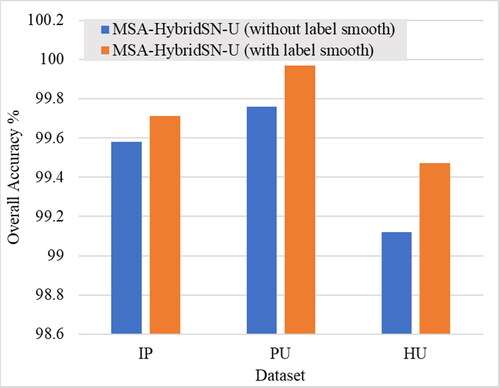
Figure 11. OA (%) of the proposed model with and without using multiscale features in the three datasets.

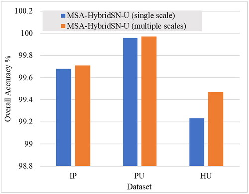
Figure 12. OA (%) of the proposed model with different attention methods in the three datasets.

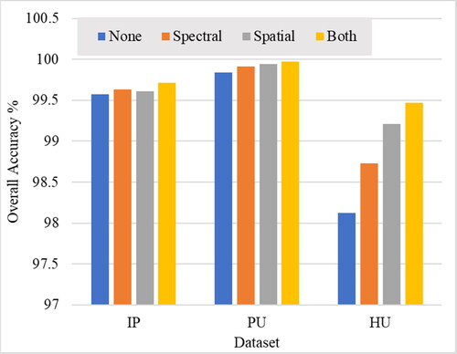
Figure 13. OA (%) of the proposed model with and without unsampled pixel utilization in the three datasets.

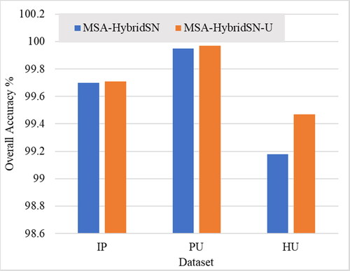
Table 10. Effect of training sample size on the proposed model for hyperspectral image classification.

IP Dataset
Training Sample Size (%)	OA	AA	Kappa
5	99.71	99.65	0.997
10	99.82	99.76	0.998
20	99.91	99.85	0.999
50	99.98	99.92	1
70	99.99	99.93	1
PU Dataset
5	99.97	99.89	0.999
10	99.97	99.89	0.999
20	99.99	99.93	1
50	1	1	1
70	1	1	1
HU Dataset
5	99.47	99.92	0.994
10	99.51	99.96	0.995
20	99.73	99.98	0.997
50	99.94	99.99	0.999
70	99.98	99.99	1

The table shows the OA, AA, and Kappa for three benchmark datasets: IP, PU, and HU.

Table 11. Computational complexity (training time and test time) of the proposed and benchmark models for hyperspectral image classification based on the IP dataset.

Model	Training Time (minutes)	Test Time (seconds)
SVM	22	7
2D CNN	17	8
3D CNN	32	13
HybridSN	26	10
M3D-DCNN	24	12
DBDA	28	13
ACA-HybridSN	30	12
MSA-HybridSN-U	43	15

Data availability statement

The data that support the findings of this study are available from the corresponding author, Helmi Z. M. Shafri, upon reasonable request.