Graph neural network method for the intelligent selection of river system

Figures & data

Figure 1. Overall framework of the proposed approach for river network selection.

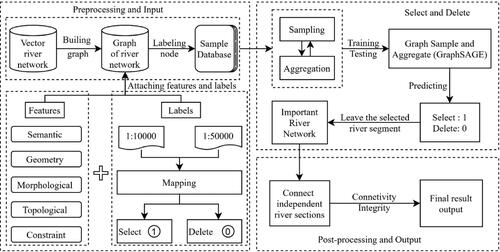
Figure 2. Graph modelling of a river network. (a) River network abstract dual graph representation; (b) primal river network; and (c) river network dual graph.

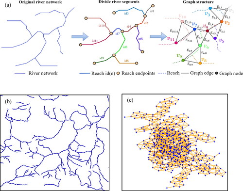
Figure 3. Example of a river network matching result. (a) 1:10,000 scale river network data; (b) 1:50,000 scale river network data; and (c) matching result.

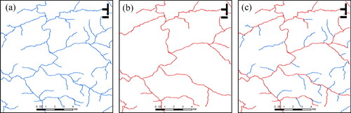
Table 1. Graph node characteristics.

Feature item		Description
Semantic feature	River order	Reflects importance: the higher the grade, the more important the river segment.
Geometric feature	River segment length	Reflects influence: the longer the river segment, the greater the scope of influence.
Morphological feature	River curvature	Reflects the velocity of the river: the greater the curvature of the river and the longer the length, the lower the velocity (because the water is spread over a larger area, the river flows less).
Topological features	Number of adjacent nodes	Reflects the upstream and downstream connections of the river segment: the more adjacent nodes in the graph structure, the more connected the river segment.
	Number of adjacent lakes	Reflects the developed hydrological system of the basin: the greater number of lakes, the more developed the hydrological system around the basin, which provides more water resources.
Binding feature	1:25,000 river network	Reflects the constraints of the network: a 1:25,000 scale river network of the same area is used to constrain and ensure the spatial consistency of the geographical elements.

Figure 4. River network selection sample coding. (a) Sample initial features; and (b) sample encoded features.

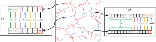
Figure 5. River network neighbour sampling and aggregation. (a) Sample neighbourhood; (b) aggregate feature information from neighbours; and (c) categorisation using aggregated information.

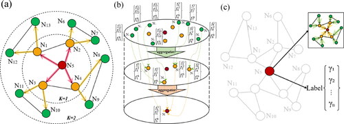
Figure 6. Graph classification model based on GraphSAGE, which contains two convolutional layers (SAGEConv): a fully connected layer (linear) and a normalised exponential layer (Softmax).

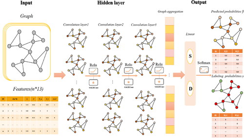
Figure 7. Experimental data: (a) 1:10,000 and 1:50,000 overlays; (b) 1:10,000 partial area; and (c) 1:50,000 partial area.

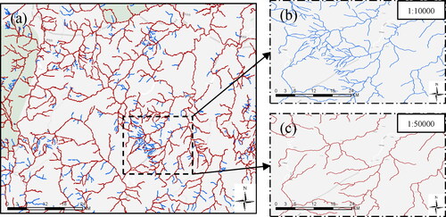
Figure 8. Loss value and accuracy curves of neural network models in different graphs. (a) Loss value change curve of different models; and (b) validation dataset accuracy curve of different models.

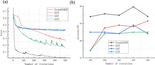
Figure 9. Influence of the number of node features on accuracy.

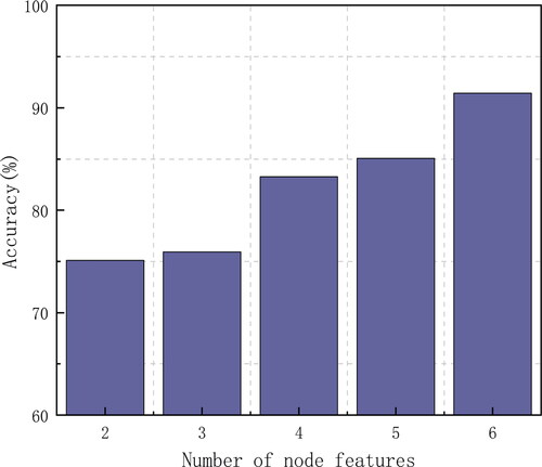
Figure 10. Influence of different hyperparameters on the accuracy of the model.

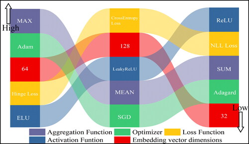
Figure 11. Accuracy and loss values of different depth models.

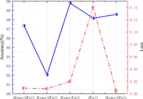
Table 2. Test set classification result statistics.

Evaluation index	TP	FP	FN	TN
	218	5	0	50
	Acc (%)	Pre (%)	Rec (%)	F1_Score (%)
	98.17	98.63	99.08	98.86

Figure 12. Accuracy of the compared methods.

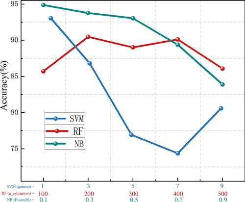
Table 3. Comparison of classification accuracy among similar algorithms.

Index	GraphSAGE	SVM	RF	NB
Accuracy (%)	98.17	93.04	90.47	94.87

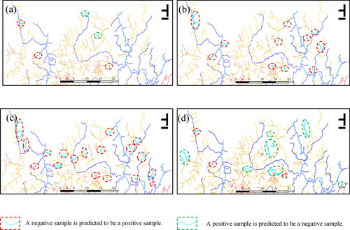
Figure 13. Incorrect results predicted by different classification methods. (a) Misclassified river segment by GraphSAGE. (b) Misclassified river segment by NB. (c) Misclassified river segment by RF. (d) Misclassified river segment by SVM.

Data availability statement

The data and codes that support the findings of this study are available in Figshare at https://doi.org/10.6084/m9.figshare.22793993.v1