Are public green spaces distributed fairly? A nationwide analysis based on remote sensing, OpenStreetMap and census data

Figures & data

Figure 1. Workflow of this study. The GLC dataset is derived from a land cover classification (*) developed by Weigand et al. (2020) and PGS is derived from a deep learning data fusion (see sec. 3.1.2). both datasets are used in conjunction with nationwide census data to support the analyses in this study.

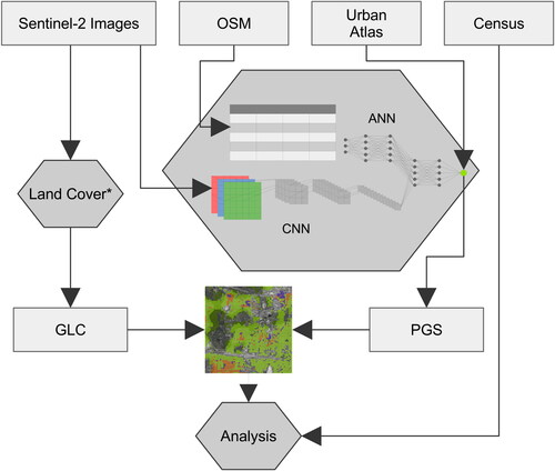
Table 1. Aggregation scheme for census building type classification.

Aggregated type	N Cells	Census building type
Detached house	716949	Detached single-family home
		Detached two-family home
Semi-detached house	42066	Semi-detached single-family home
		Semi-detached two-family home
Terraced house	34425	Terraced single-family home
		Terraced two-family home
Multi-family home	22214	Multi-family home 3 - 6 flats
		Multi-family home 7 - 12 flats
		Multi-family home 13 flats or more

For each aggregated class, the number of neighbourhoods (N cells) with buildings of exclusively one aggregated building type and at least 5 buildings are summarized.

Figure 2. Availability of neighbourhood GLC and PGS in Germany by cumulative shares of the population. The separate plots use different grouping variables: A) Entire Germany, B) by municipality size in by population in thousands (K), C) by the 5-class rural urban gradient by Taubenböck et al. (2022), and D) in neighbourhoods with specific building types.

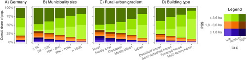
Figure 3. Green space availability in Germany by federal states. States are shaded by the population-weighted average of PGS available. Pie charts indicate the distribution of PGS and GLC, the colors follow the legend in Figure 2.

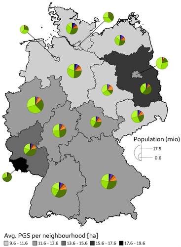
Figure 4. Equity of GLC (pink) and PGS (green) availability in Germany at national, regional and city level. A) depicts a lorenz curve showing the availability of the resources in Germany. Point plots visualize the distribution of Gini coefficients measuring distributive equity of the resources in different spatial samples: B) by the municipality size denoted in classes of thousands (K) of inhabitants per municipality, C) by the neighbourhood classification along the rural-urban gradient, and D) by neighbourhoods with distinct housing types. For reference, the horizontal lines in B), C), and D) visualize the Gini coefficient per resource for the entire population of Germany.

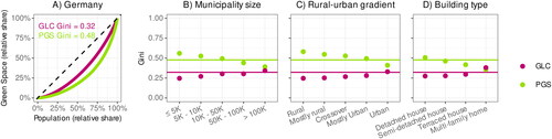
Figure 5. Comparison of green space availability by cumulative population share (coloured bars) and PGS Gini coefficient (black dots) for the 100 most populated cities in Germany. The colours follow the legend in Figure 2. The cities are ranked by the proportion of the population that has more than 3.6 hectares of the PGS in the neighbourhood which is the WHO target (green coloured bars). the main findings include: the range of population with above-target PGS values varies significantly among the largest cities, the PGS Gini coefficient only weakly correlates with the PGS above-target population shares (r = -0.52) with distinct outliers like darmstadt or heilbronn.

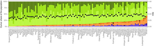
Table 2. LMM estimated fixed effects (FE) and random effects (RE) modelling the relation between green land cover (GLC, in ha.) and population (log.), the share of foreigners, children, and elderly across populated 1 km $\times$ 1 km grid cells in Germany.

	GLC (1)	GLC (2)	GLC (3)	GLC (4)	GLC (5)
Intercept FE	64.854^***	65.266^***	65.014^***	64.708^***	63.050^***
log(pop.) FE	−2.544^***	−2.766^***	−2.815^***	−2.754^***	−2.750^***
share foreign. FE	−0.195^***			−0.226^***	−0.224^***
share children FE		0.018^***		0.033^***	0.033^***
share elderly FE			0.042^***	0.041^***	0.041^***
Municip. RE	✓	✓	✓	✓	✓
City size class RE					✓
Rural-urban grad. RE
Model R^2	0.618	0.621	0.621	0.624	0.624
N cells	211,271	204,091	198,740	174,126	174,126
	GLC (6)	GLC (7)	GLC (8)	GLC (9)
Intercept FE	62.989^***	62.624^***	59.470^***	59.213^***
log(pop.) FE	−2.687^***	−2.688^***	−2.663^***	−2.530^***
share foreign. FE	−0.208^***	−0.208^***	−0.028^**	−0.003
share children FE	0.030^***	0.030^***	0.102^***	0.092^***
share elderly FE	0.040^***	0.040^***	0.069^***	0.066^***
Municip. RE	✓	✓
City size class RE		✓	✓
Rural-urban grad. RE	✓	✓		✓
Model R^2	0.626	0.626	0.050	0.053
N cells	174,091	174,091	174,126	174,091

Significance levels ^***p-value < 0.001,^**p-value < 0.01.

Table 3. LMM estimated fixed effects (FE) and random effects (RE) modelling the relation between public green space (PGS, in ha.) and population (log.), the share of foreigners, children, and elderly across populated 1 km × 1 km grid cells in Germany.

	PGS (1)	PGS (2)	PGS (3)	PGS (4)	PGS (5)
Intercept FE	30.998^***	31.533^***	30.833^***	31.127^***	32.978^***
log(pop.) FE	−3.066^***	−2.888^***	−3.072^***	−2.877^***	−2.885^***
share foreign. FE	0.048^***			0.042^***	0.039^***
share children FE		−0.074^***		−0.082^***	−0.082^***
share elderly FE			0.021^***	0.018^***	0.017^***
Municip. RE	✓	✓	✓	✓	✓
City size class RE					✓
Rural-urban grad. RE
Model R ^2	0.456	0.459	0.457	0.455	0.455
N cells	211,271	204,091	198,740	174,126	174,126
	PGS (6)	PGS (7)	PGS (8)	PGS (9)
Intercept FE	31.835^***	32.809^***	30.775^***	30.520^***
log(pop.) FE	−2.896^***	−2.895^***	−2.519^***	−2.575^***
share foreign. FE	0.037^***	0.036^***	0.141^***	0.128^***
share children FE	−0.082^***	−0.082^***	−0.113^***	−0.114^***
share elderly FE	0.018^***	0.017^***	0.035^***	0.034^***
Municip. RE	✓	✓
City size class RE		✓	✓
Rural-urban grad. RE	✓	✓		✓
Model R ^2	0.455	0.455	0.067	0.069
N cells	174,091	174,091	174,126	174,091

Significance levels^***p-value < 0.001,^**p-value < 0.01.

Table 4. LMM estimated fixed effects (FE) and random effects (RE) modelling the relation between green land cover (GLC, in ha.) and population (log.), the share of foreigners, children, and elderly across populated 1 km × 1 km grid cells in Germany.

	GLC (1)	GLC (2)	GLC (3)	GLC (4)	GLC (5)
Intercept FE	59.726^***	63.079^***	62.946^***	64.989^***	63.731^***
log(pop.) FE	−1.176^***	−2.109^***	−2.646^***	−3.525^***	−4.783^***
share foreign. FE	0.102^***	−0.054^***	−0.137^***	−0.185^***	−0.327^***
share children FE	−0.011	−0.022^*	0.011	0.029^*	0.206^***
share elderly FE	0.017^**	0.015^**	0.052^***	0.065^***	0.255^***
Rural-urban class	Rural	Mostly rural	Crossover	Mostly Urban	Urban
Municip. RE	✓	✓	✓	✓	✓
Model R ^2	0.730	0.661	0.625	0.586	0.497
N cells	28,768	64,168	41,665	22,836	16,654

Significance levels^***p-value < 0.001,^**p-value < 0.01,^*p-value < 0.05.

Table 5. LMM estimated fixed effects (FE) and random effects (RE) modelling the relation between public green space (PGS, in ha.) and population (log.), the share of foreigners, children, and elderly across populated 1 km × 1 km grid cells in Germany.

	PGS (1)	PGS (2)	PGS (3)	PGS (4)	PGS (5)
Intercept FE	29.683^***	33.789^***	30.997^***	32.449^***	30.577^***
log(pop.) FE	−2.958^***	−3.336^***	−2.640^***	−2.538^***	−2.474^***
share foreign. FE	0.121^***	0.086^***	0.081^***	0.000	−0.016
share children FE	−0.032^***	−0.076^***	−0.077^***	−0.099^***	−0.067^***
share elderly FE	0.007	0.008.	0.038^***	0.025^**	0.108^***
Rural-urban class	Rural	Mostly rural	Crossover	Mostly Urban	Urban
Municip. RE	✓	✓	✓	✓	✓
Model R ^2	0.622	0.483	0.433	0.463	0.361
N cells	28,768	64,168	41,665	22,836	16,654

Significance levels^***p-value < 0.001,^**p-value < 0.01,^*p-value < 0.05,. p-value < 0.1.

Weigand M, Staab J, Wurm M, Taubenböck H. 2020. Spatial and semantic effects of LUCAS samples on fully automated land use/land cover classification in high-resolution Sentinel-2 data. Int J Appl Earth Obs Geoinf. 88(:102065. doi: 10.1016/j.jag.2020.102065.

 Web of Science ®Google Scholar

Taubenböck H, Droin A, Standfuß I, Dosch F, Sander N, Milbert A, Eichfuss S, Wurm M. 2022. To be, or not to be ‘urban’? A multi-modal method for the differentiated measurement of the degree of urbanization. Comput Environ Urban Syst. 95:101830. doi: 10.1016/j.compenvurbsys.2022.101830.

 Web of Science ®Google Scholar

Data availability statement

Data available from the authors on request. The code used for this study is published at https://github.com/dlr-eoc/ukis-paperfairgreen.