Figures & data
Figure 1 Schematic figure of an EDL near a negatively charged planar surface. The water dipoles in the vicinity of the charged surface are partially oriented towards the surface.
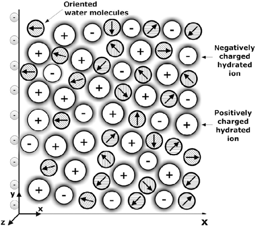
Figure 2 Relative permittivity (Equation (38)) as a function of the distance from the charged surface x within the LB model for finite-sized ions. Three values of surface charge density were considered:
,
and
. Equation (36) was solved numerically as described in the text. The dipole moment of water
, bulk concentration of salt
, bulk concentration of water
, where
is the Avogadro number.
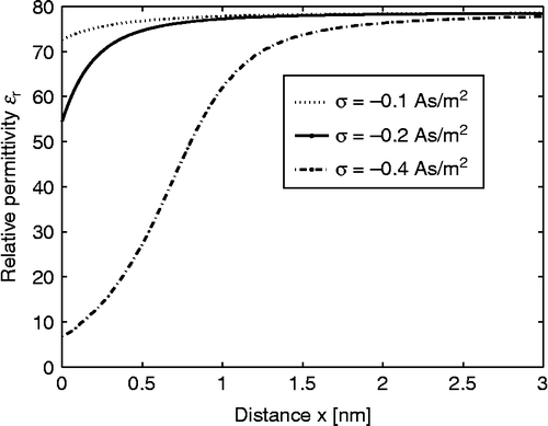
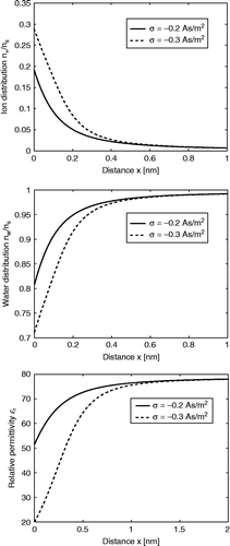
Figure 3 The relative number density of counter ions and water Langevin dipoles
as a function of the distance from the charged surface x (calculated using Equations (21) and (23), respectively) within the LB model for finite-sized ions. Three values of surface charge density were considered:
,
and
. Equation (36) was solved numerically as described in the text. The other values of the model parameters are the same as in Figure 2.
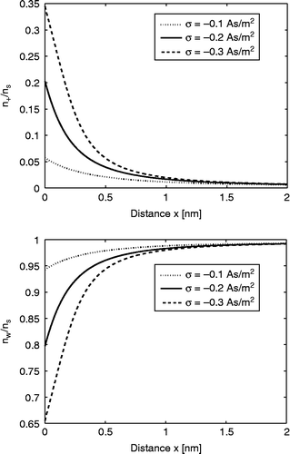
Figure 4 Relative dielectric permittivity (Equation (69)) as a function of the distance from the charged surface x within the LPB model for point-like ions. Three values of surface charge density were considered:
, σ = − 0.2 As/m2 and
. The LPB equation (67) was solved numerically as described in the text. The dipole moment of water
, bulk concentration of salt
, bulk concentration of water
, where
is the Avogadro number.
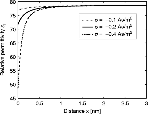
Figure 5 Electric potential as a function of the distance from the charged planar surface x within the LPB model for point-like ions (upper figure) and within the LB model for finite-sized ions (lower figure) for three values of the surface charge density;
,
and
. The dipole moment of water
, bulk concentration of salt
and bulk concentration of water
.
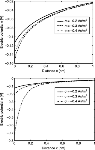
Figure 6 Charge distribution SLB model (CitationGongadze et al. 2011c), where in the interval is the region of strong water orientation and b is the distance of closest approach. The surface charge density
incorporates the negatively charged metallic surface, as well as the specifically bound negatively charged ions (CitationButt et al. 2003).
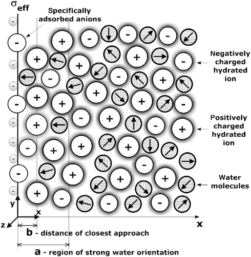
Figure 7 Electric potential as a function of the distance from the charged planar surface x (
) within the Stern model (Equation (77)), the SLPB model for point-like ions (Equation (79)), the SLB model for finite-sized ions (Equation (81)) and the SLB model with a step function for finite-sized ions (Equation (83)) for c = 0, where in all four cases the distance of closest approach
was taken into account. The value of the surface charge density was considered to be:
(upper figure) and
(lower figure). The remaining parameters used are dipole moment of water,
; bulk concentration of salt,
and bulk concentration of water,
, where
is Avogadro number.
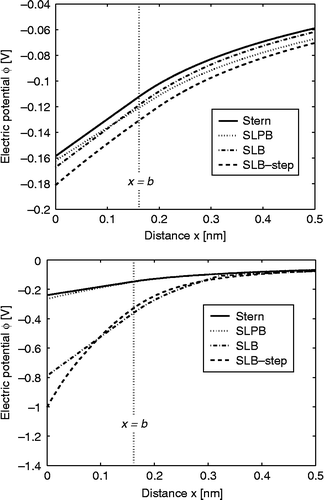
Figure 8 Relative permittivity as a function of the magnitude of electric field strength (E) within the LPB model (Equation (69)) and BLP model (Equation (93)) for point-like ions and
, where
is the Avogadro number. In the case of the LPB model, the effective dipole moment of water
, while in the BLP model the dipole moment of water
and
.
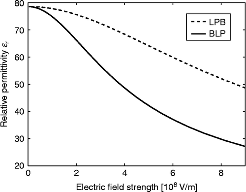
Figure 9 The relative number density of counter ions , water dipoles
(calculated using Equations (111) and Equation (113) and relative permittivity
(Equation (117)) as a function of distance from a planar-charged surface x (adapted from CitationGongadze and Iglič 2012). Two values of surface charge density were considered:
and
. Equation (118) was solved numerically taking into account the boundary conditions (120) and (121) as described in the text. Values of parameters assumed are dipole moment of water,
; bulk concentration of salt,
; optical refractive index,
; bulk concentration of water,
, where
is Avogadro number.