An in vivo parameter identification method for arteries: numerical validation for the human abdominal aorta

Figures & data

Figure 1. Stress-free $\left({\mathcal{B}}_0\right)$, unloaded $\left({\mathcal{B}}^{*}\right)$ and deformed $\left(\mathcal{B}\right)$ configuration of an arterial segment. For explanation of the parameters see Section 2.

Table 1. Parameter sets representing the created in silico arteries. The regular LH-sets, numbered 1–8, and the C-sets, numbered 9–17, are taken from Labrosse et al. (2013) and Horný et al. (2014). The set numbers within brackets refer to the naming convention in Horný et al. (2014). The sets numbered 18–22 are the artificial A-sets. Note that the reduced axial force ${\widehat{F}}_{\text{red}}$ is stated as its mean value of the corresponding thick-walled FE model.

		Labrosse et al. (2013)			Horný et al. (2014)				Computed		Agreement
		$R_{\mathrm{i}}$	H	${\Phi }_0$	c	k1	k2	β	λz	${\widehat{F}}_{\text{red}}$	$R^2$	RMSE
	Set	[mm]	[mm]	[deg]	[kPa]	[kPa]	[-]	[deg]	[-]	[N]	[-]	[mm]
LH-sets	1 (F49)	5.9	1.51	252.00	2.31	20.06	4.11	39.95	1.1699	0.57	0.63	0.08
	2 (F63)	5.4	0.96	96.00	13.59	41.78	3.29	39.86	1.1594	0.74	0.97	0.03
	3 (M38)	5.3	1.22	117.00	12.20	19.28	3.22	41.60	1.1576	0.74	0.88	0.06
	4 (M60)	6.3	1.69	156.00	5.91	17.57	3.18	43.16	1.1217	0.83	0.72	0.10
	5 (M61b)	7.3	1.62	335.00	6.98	11.37	8.05	41.95	1.1039	0.67	0.52	0.07
	6 (M66)	7.2	1.78	253.00	17.78	25.72	7.65	38.85	1.1385	1.49	0.90	0.04
	7 (M70a)	7.1	1.23	208.00	2.78	67.45	7.02	35.49	1.1908	0.60	0.95	0.03
	8 (M70b)	7.4	1.64	201.00	12.18	17.31	22.86	39.69	1.0582	0.52	0.53	0.05
C-sets	9 (F50)	6.7	1.14	323.00	0.68	49.54	7.44	36.67	1.1791	0.41	0	4.27
	10 (F65)	6.2	1.21	248.00	0.05	9.06	5.87	39.36	1.1932	0.36	0	0.76
	11 (M42)	6.5	1.56	125.00	0.22	21.88	0.62	38.34	1.4322	1.52	0.93	0.09
	12 (M57)	7.5	1.28	322.00	0.05	4.37	4.87	41.11	1.2080	0.55	0	0.61
	13 (M61a)	7.7	1.22	270.00	0.05	49.45	26.74	37.55	1.0836	0.25	0	0.73
	14 (M67a)	8.0	1.58	118.00	0.05	41.95	22.00	38.18	1.0666	0.34	0	1.54
	15 (M67b)	7.9	1.26	174.00	0.05	61.02	7.02	35.49	1.1984	0.56	0	0.49
	16 (M71)	10.0	1.72	118.00	0.05	94.49	9.26	37.65	1.0964	0.84	0	0.70
	17 (M77)	7.0	1.50	135.00	0.05	26.65	39.30	38.23	1.0500	0.19	0	1.39
A-sets	18	10.1	2.81	46.19	32.68	7.44	47.90	40.02	1.0210	0.65	0.34	0.10
	19	14.9	2.81	52.23	67.39	22.53	11.79	47.47	1.0489	5.95	1.0	0.03
	20	5.3	1.41	20.98	75.91	71.16	67.08	37.06	1.0422	1.03	0.96	0.01
	21	3.9	0.68	28.81	90.87	64.35	38.12	39.34	1.0281	0.29	0.99	0.00
	22	12.3	3.54	81.75	28.89	21.33	3.29	53.24	1.0372	3.18	0.98	0.12

Table 2. Fitting ranges of the structural and material parameters of the AA.

Parameter	$R_{\mathrm{i}}$	λz	c	k1	k2	β
	[mm]	[-]	[kPa]	[kPa]	[-]	[deg]
${\mathit{\kappa }}_{\text{min}}$	0.1	1	$1·{10}^{-7}$	$1·{10}^{-7}$	$1·{10}^{-4}$	0
${\mathit{\kappa }}_{\text{max}}$	25	10	$3·{10}^3$	$6·{10}^3$	$4·{10}^3$	90

Table 3. Mean difference and 95% limits of agreement of identified and FE values for the verification.

		LH- and A-sets		C-sets
Parameter	Unit	Mean difference	95% limits of agreement	Mean difference	95% limits of agreement
$R_{\mathrm{i}}$	[mm]	0.002	–0.007 to 0.011	0.25	–1.01 to 1.53
λz	[-]	–0.001	–0.002 to 0.001	0.51	–1.53 to 2.54
c	[kPa]	0.034	–0.017 to 0.085	0.02	–0.07 to 0.11
k1	[kPa]	0.075	–0.110 to 0.259	0.67	–0.23 to 1.57
k2	[-]	0.026	–0.043 to 0.094	0.13	–0.13 to 0.46
β	[deg]	0.008	–0.049 to 0.065	–5.67	–30.14 to 18.80

Table 4. Mean difference and 95% limits of agreement of identified and FE values for the validation.

		LH- and A-sets		C-sets
Parameter	Unit	Mean difference	95% limits of agreement	Mean difference	95% limits of agreement
$R_{\mathrm{i}}$	[mm]	0.09	–0.34 to 0.52	0.14	–1.27 to 1.55
λz	[-]	0.04	–0.13 to 0.20	2.50	–0.42 to 5.41
c	[kPa]	0.36	–1.80 to 2.51	0.99	–2.29 to 4.27
k1	[kPa]	–0.01	–10.23 to 10.21	3.68	–24.69 to 32.05
k2	[-]	0.98*	0.75 to 1.21*	1.10*	0.41 to 1.78*
β	[deg]	–3.80	–9.97 to 2.37	–22.56	–51.87 to 6.76

*Mean ratio and the corresponding 95% limits of agreement are presented instead.

Figure 7. Comparison of predicted (red dotted line) with validation pressure-radius data (black dashed line) for parameter sets 2, 15 and 18 from Table 1.

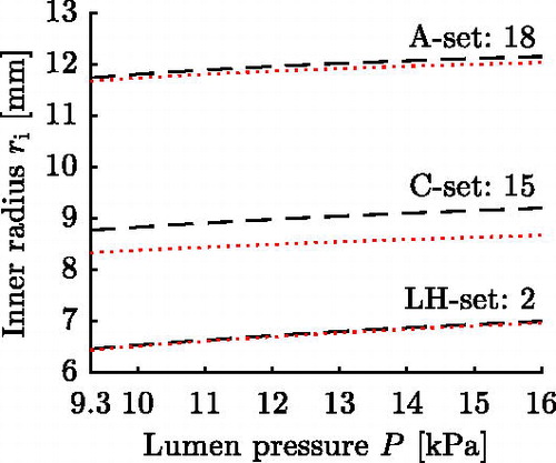
Figure 2. Circumferential stretch for the pressures 9.3, 13.3 and $16 \text{kPa}$ for parameter set 18 from Table 1.

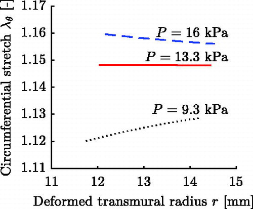
Figure 3. Examples of meshes for two different FE models of an AA.

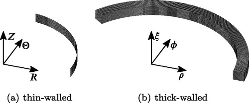
Figure 4. Reduced axial force for three different axial prestretches for parameter set 18 from Table 1.

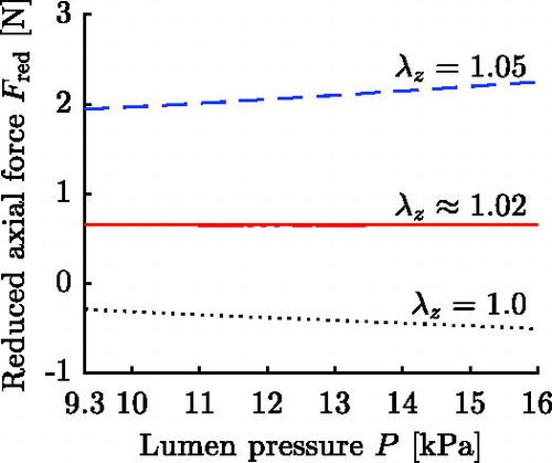
Figure 5. Difference between identified and FE values plotted against the FE values for each parameter of the verification sets. The solid black lines represents perfect agreement, the dotted red line is the mean difference and the dashed red lines denote the 95% limits of agreement of the LH- and A-sets. Note that a logarithmic abscissa is used for parameters c and k₂.

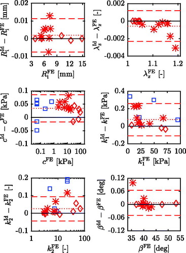
Figure 6. Difference between identified and FE values plotted against the FE values for each parameter of the validation sets. The solid black lines represents perfect agreement, the dotted red line is the mean difference and the dashed red lines denote the 95% limits of agreement of the LH- and A-sets. Note that for parameter k₂ the ordinate shows the ratio of identified and pre-defined value and a logarithmic abscissa is used for parameters c and k₂.

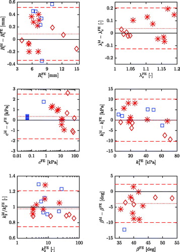
Figure A1. Example geometries of the arterial segment for different opening angles. For explanation of the parameters see Appendix A.

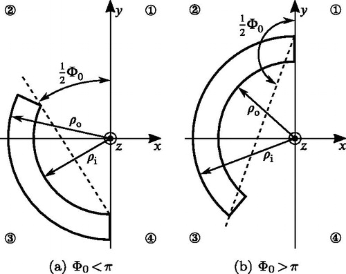
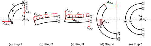
Figure A2. BCs of the different simulation steps illustrated for an artery with ${\Phi }_0>\pi$. For explanation of the parameters see Appendix A.

Labrosse MR, Gerson ER, Veinot JP, Beller CJ. 2013. Mechanical characterization of human aortas from pressurization testing and a paradigm shift for circumferential residual stress. J Mech Behav Biomed Mater. 17:44–55.

 PubMed Web of Science ®Google Scholar

Horný L, Netušil M, Daniel M. 2014. Limiting extensibility constitutive model with distributed fibre orientations and ageing of abdominal aorta. J Mech Behav Biomed Mater. 38:39–51.

 PubMed Web of Science ®Google Scholar