Figures & data
Figure 1. Vertical component of a GRF signal. Ordinate corresponds to newtons normalized by weight of the runner. The active peak corresponds to the value of 250%, where 100% means the body weight of the runner. Abscissa corresponds to frames in a way that there is one data point per frame, 300 frames per second. On the left plot GRF peak without protruding impact peak is presented. On the right plot is GRF peak with protruding impact peak.
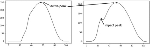
Figure 2. Anthropometric data of the subjects. In the first row: bodyweight (kg), height (cm); in the second row: average leg length (cm), body mass index (kg/m2). The values on each plot are sorted from the smallest to the greatest independently from the other plots after the calculation of body mass index.
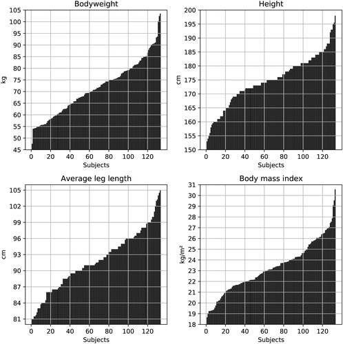
Figure 3. Location of the markers employed (according to standard Vicon plug-in gait lower body model1). RPSI, LPSI, RHEE, and RHEE markers’ location is on the back side of the body, thus they are marked with gray color. Credit (Taylor Citation2012).
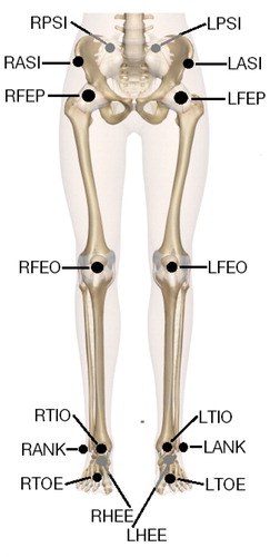
Figure 4. A scheme of a convolutional part of the neural network models.
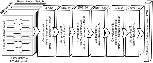
Table 1. A list of classifiers employed and their training parameters (default if not mentioned).
Table 2. Performance of the models.
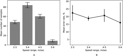
Figure 5. A bar plot A represents mean number of samples over the cross-validated test folds against speed ranges. A plot B represents mean error rate values over the cross-validated test folds for each range of speed. Error rate was calculated as a sum of false positive and false negative predictions divided by the total amount of the predictions. The random forest model was employed to obtain predictions.