Overset meshing in combination with novel blended weak-strong fluid-structure interactions for simulations of a translating valve in series with a second valve

Figures & data

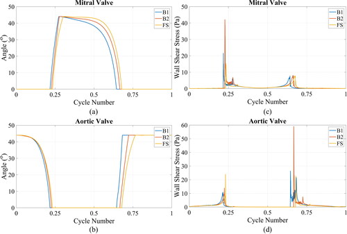
Figure 1. Outline of the computational domain (a) Full domain geometry with fluid cylinder and two BMHVs (b) 1/4 domain geometry: yz-symmetry (red), yx-symmetry (green) (c) Angle of leaflet in closed and open positions (d) Monitor point location with inlet, outlet, and wall boundaries.

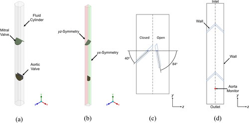
Figure 2. Fluid mesh definition (a) Fluid mesh zones: mitral component zone (blue), aortic component zone (green), background zone (grey), collar zones (red) (b) before and after initialisation of whole mesh (c) before and after initialisation of mitral mesh zone.

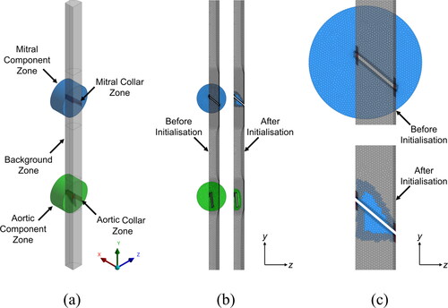
Table 1. Mesh densities of the three meshes used in the mesh convergence study.

	Mesh Density	Tetrahedral Element Count	Polyhedral Element Count
1	Coarse	0.84M	0.28M
2	Medium	1.2M	0.4M
3	Fine	2.1M	0.7M

Figure 3. Solution strategy flow diagram. Rectangular boxes represent processes, diamond boxes represent decisions, parallelograms represent input/output. Arrows are the flow of logic through the strategy. n is the time step number, k is the iteration number, and $T_{\mathit{\text{END}}}$ is the end time of the solution.

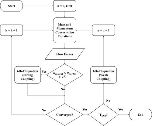
Table 2. Variable time stepping scheme conditions. Two conditions depend on moving and stationary valves. When valves are moving, two sub conditions interrogate the leaflet angle, and adjust the time step accordingly.

Number	Condition		Timestep Size
1 (Moving)	$\left|{\omega }_{\mathit{\text{mitral}}}\right|>0$ or $\left|{\omega }_{\mathit{\text{aortic}}}\right|>0$	${\theta }_{\mathit{\text{mitral}}}>2°$ or ${\theta }_{\mathit{\text{aortic}}}>2°$	$\mathit{\text{dt}}=\mathrm{\text{min}}\hspace{0.17em}\left(\frac{0.5°}{{\omega }_{\mathit{\text{mitral}}}},\frac{0.5°}{{\omega }_{\mathit{\text{aortic}}}},2.5\mathit{\text{ ms }}\right)$
		${\theta }_{\mathit{\text{mitral}}}<2°$ and ${\theta }_{\mathit{\text{aortic}}}<2°$	$\mathit{\text{dt}}=\mathrm{\text{min}}(\frac{0.1°}{{\omega }_{\mathit{\text{mitral}}}},\frac{0.1°}{{\omega }_{\mathit{\text{aortic}}}})$
2 (Stationary)	${\omega }_{\mathit{\text{mitral}}}=0$ and ${\omega }_{\mathit{\text{aortic}}}=0$		$\mathit{\text{dt}}=2.5 \mathit{\text{ms}}$

Figure 4. Variation in $\theta$ over time for the coarse, medium, and fine meshes for the (a) mitral and (b) aortic valves.

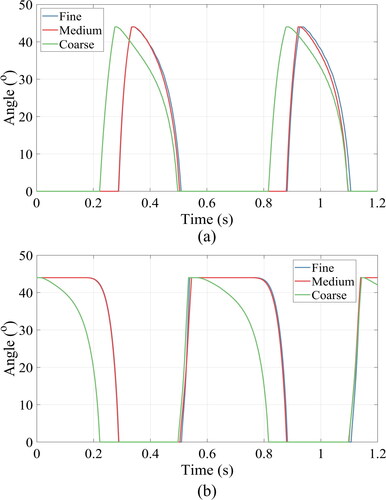
Figure 5. Variation in $\overline{\mathit{\text{WSS}}}$ over time for the coarse, medium and fine meshes for the (a) mitral and (b) aortic valves.

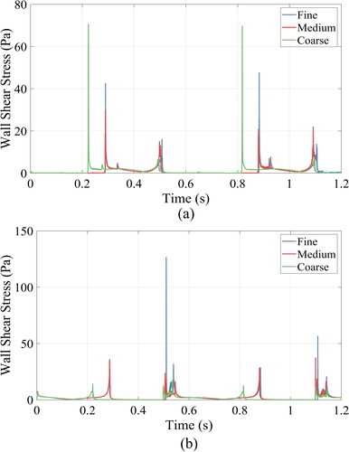
Figure 6. Variability in time step size and $\theta$ for the mitral and aortic valves, showing the effect of the variable time stepping scheme outlined in Table 2.

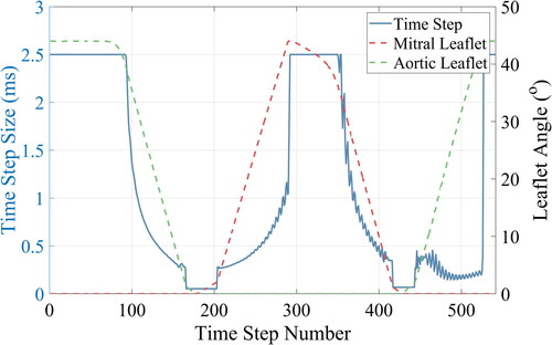
Figure 7. Velocity magnitude and pressure contours when leaflet angle is $\theta =44°$ (fully open) for a change in stroke length and stroke rate. Note the scaling of the velocity magnitude contours is 0-0.3 m s⁻¹ for the 25 mm stroke length cases, and 0-0.6 m s⁻¹ for the 50 mm stroke length cases. Velocity magnitude contour plots are clipped to the maximum values of 0.3 m s⁻¹ and 0.6 m s⁻¹ in each of the cases respectively.

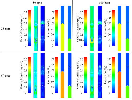
Figure 8. Valve motion over final cycle alongside AV plane displacement for the (a) mitral valve and (b) aortic valve.

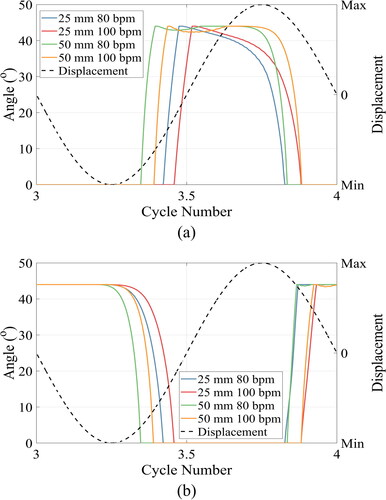
Figure 9. Change in (a) ${\omega }_{\mathit{\text{closing}}}$ and (b) ${\omega }_{\mathit{\text{opening}}}$ for the mitral and aortic valve leaflets with a change in stroke length and stroke rate.

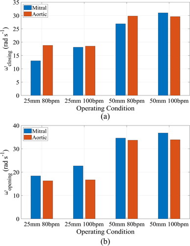
Figure 10. Variation in aortic pressure with a change in stroke length and stroke rate. Time frame limited between cycle number 1.75 and 2.75 to highlight variation during full range of aortic valve motion. Vertical lines correspond to instantaneous pressure spikes.

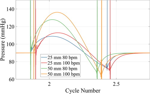
Figure 11. Variation in $\overline{\mathit{\text{WSS}}}$ over the course of the last cycle for the (a) Mitral valve and (b) Aortic Valve.

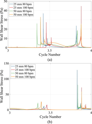
Figure 12. Contour plot of wall shear values on surface of (a-d) aortic valve leaflet and (e-h) mitral valve leaflet when leaflet angle is $\mathrm{\theta }=44°$ (fully open), for a change in stroke length and stroke rate. Note a difference in scaling between individual contour images.

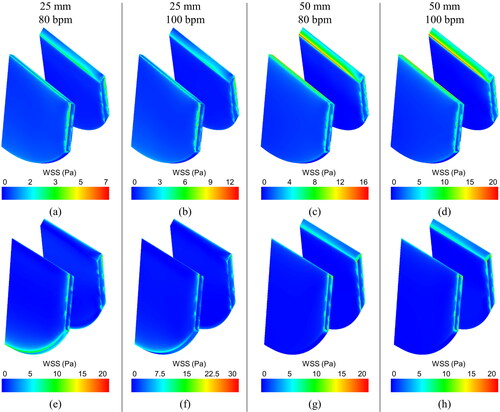
Table 3. $\overline{\mathit{\text{TAWSS}}}$ values for a variation in stroke length and stroke rate.

	25 mm/ 80 bpm	25 mm/ 100 bpm	50 mm/ 80 bpm	50 mm/ 100 bpm
${\overline{\mathit{\text{TAWS}}}}_{\mathit{\text{mitral}}}$	0.80	1.08	1.89	2.31
${\overline{\mathit{\text{TAWS}}}}_{\mathit{\text{aortic}}}$	1.16	1.50	1.98	2.32

Figure 13. (a) Variation in $Q_{\mathit{\text{inlet}}}$ for all four cycles with a variation in stroke length and stroke rate (b) Cumulative outlet flow over the four cycles.

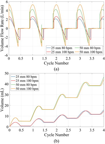
Figure 14. Variation in (a) volume flow and (b) volume flow rate through the outlet for a change in stroke length and stroke rate.

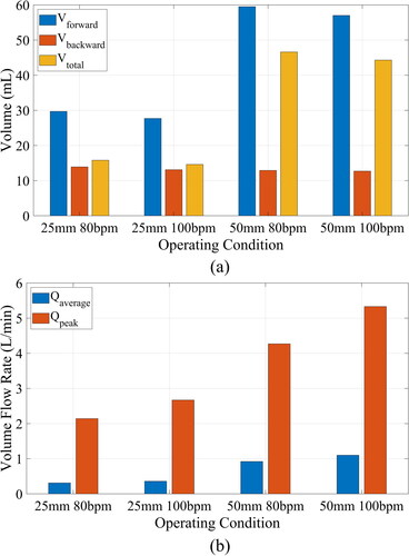
Figure 15. Comparison of blended scheme 1 (B1), blended scheme 2 (B2) and fully strongly coupled (FS) schemes for (a) mitral valve leaflet angle, (b) aortic valve leaflet angle, (c) mitral valve $\overline{\mathit{\text{WSS}}}$ and (d) aortic valve $\overline{\mathit{\text{WSS}}}.$