2,563
Views
9
CrossRef citations to date
0
Altmetric
Original Articles

Condition prediction and estimation of service life in the presence of data censoring and dependent competing risks

ORCID Icon &
Pages 313-331 | Received 14 Aug 2016, Accepted 05 Feb 2017, Published online: 21 Feb 2017

Figures & data

Figure 1. Common types of censoring of the lifetime (service life) of pavements in the context of continuous condition deterioration, application of treatments and periodic condition surveys.
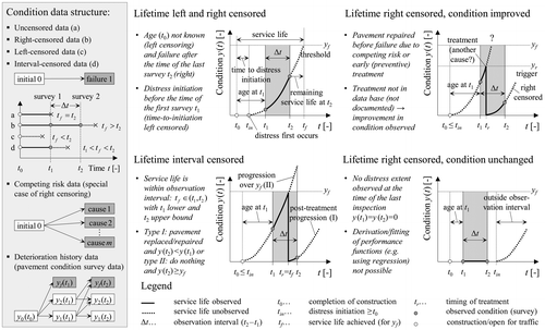
Figure 1. Common types of censoring of the lifetime (service life) of pavements in the context of continuous condition deterioration, application of treatments and periodic condition surveys.

Figure 2. Relationship between probability density, hazard and survival function (a). Parametric likelihood estimation accommodating uncensored, left-, interval- and right-censored data (b).
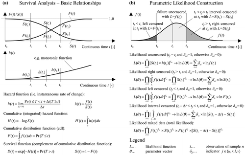
Figure 2. Relationship between probability density, hazard and survival function (a). Parametric likelihood estimation accommodating uncensored, left-, interval- and right-censored data (b).

Figure 3. Overview of classic non-parametric, semi-parametric and parametric models in survival analysis together with their characteristics and limitations.
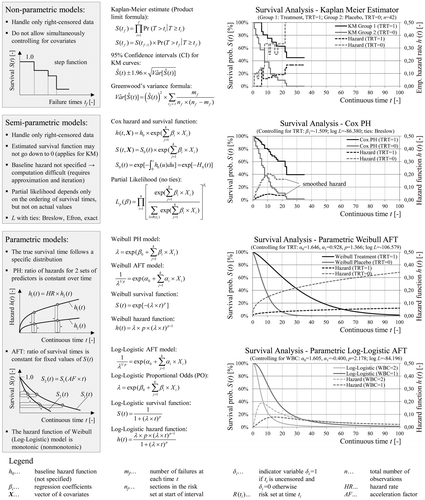
Figure 3. Overview of classic non-parametric, semi-parametric and parametric models in survival analysis together with their characteristics and limitations.

Figure 4. Data-generation procedure based on assumed service life (failure) distributions and performance functions with age as a dependent variable (a, b). Modelling of pavement cracking as a combination of two processes - initiation and progression (c, d).
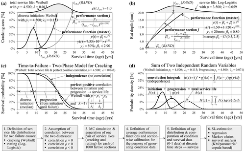
Figure 4. Data-generation procedure based on assumed service life (failure) distributions and performance functions with age as a dependent variable (a, b). Modelling of pavement cracking as a combination of two processes - initiation and progression (c, d).

Figure 5. Generation of different age distributions (uniform). Definition of survival time as time from construction until failure with the corresponding transformation to age as the time scale.
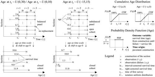
Figure 5. Generation of different age distributions (uniform). Definition of survival time as time from construction until failure with the corresponding transformation to age as the time scale.

Figure 6. Scatter-plot of the generated rutting vs. cracking survival times given the same marginal (distress-specific) distributions, but different correlation. Modelling the overall (system) pavement survival as a series system or as a composite index aggregating single distresses (standard approach).
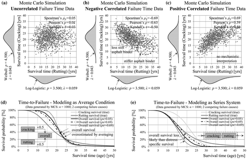
Figure 6. Scatter-plot of the generated rutting vs. cracking survival times given the same marginal (distress-specific) distributions, but different correlation. Modelling the overall (system) pavement survival as a series system or as a composite index aggregating single distresses (standard approach).

Figure 7. Estimation of performance and survival functions with non-linear regression using the generated (censored) condition data and resulting bias with respect to true marginal distributions, mean lifetimes and performance functions.
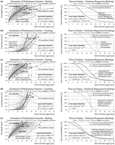
Figure 7. Estimation of performance and survival functions with non-linear regression using the generated (censored) condition data and resulting bias with respect to true marginal distributions, mean lifetimes and performance functions.

Figure 8. Relationship between survival analysis and Markov chains based on the example of a two-state (a, b) and a competing-risks (c, d) Markov chain.
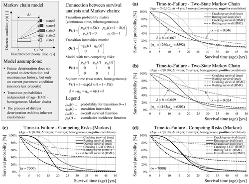
Figure 8. Relationship between survival analysis and Markov chains based on the example of a two-state (a, b) and a competing-risks (c, d) Markov chain.

Figure 9. Survival probabilities based on a five-state Markov chain with transition probabilities being constant for the full analysis period (a, b) or within age groups (c, d).
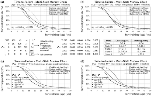
Figure 9. Survival probabilities based on a five-state Markov chain with transition probabilities being constant for the full analysis period (a, b) or within age groups (c, d).

Figure 10. KM estimates of cracking survival time in the absence of competing risks - influence of survey interval length (a), number of consecutive surveys (b), assumed lifetime distribution (c), age distribution (d) and (in)dependence of the censoring mechanism (e, f).
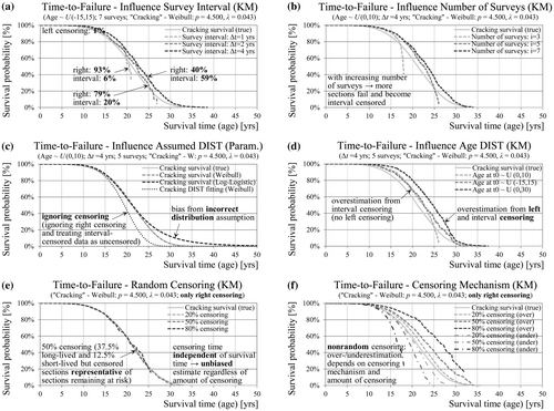
Figure 10. KM estimates of cracking survival time in the absence of competing risks - influence of survey interval length (a), number of consecutive surveys (b), assumed lifetime distribution (c), age distribution (d) and (in)dependence of the censoring mechanism (e, f).

Figure 11. Unbiased KM estimates (no interval censoring) of joint and marginal (no correlation) survival probabilities (a, b) in contrast to service life over/underestimation in the case of positive/negative correlated competing risks (c, d).
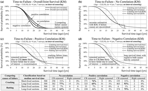
Figure 11. Unbiased KM estimates (no interval censoring) of joint and marginal (no correlation) survival probabilities (a, b) in contrast to service life over/underestimation in the case of positive/negative correlated competing risks (c, d).

Figure 12. KM/Weibull estimates of the overall (a) and marginal survival probabilities in the case of uncorrelated (b), positive (c) and negative (d) correlated cracking and rutting.
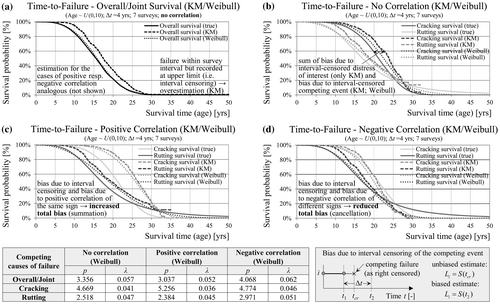
Figure 12. KM/Weibull estimates of the overall (a) and marginal survival probabilities in the case of uncorrelated (b), positive (c) and negative (d) correlated cracking and rutting.

Figure 13. Overview and estimation of cumulative incidence (a) and cumulative probability curves (b, c) based on competing risk data.
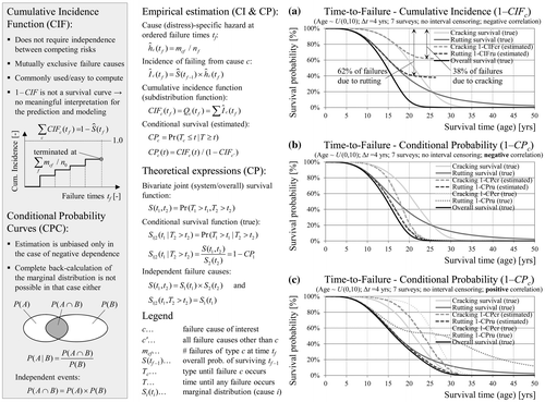
Figure 13. Overview and estimation of cumulative incidence (a) and cumulative probability curves (b, c) based on competing risk data.

Figure 14. Improvement of survival estimates for dependent competing risks by using previous conditions and distress progression models at section level in combination with survival analysis in the case of negative (a) and positive (b) correlated distresses.
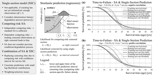
Figure 14. Improvement of survival estimates for dependent competing risks by using previous conditions and distress progression models at section level in combination with survival analysis in the case of negative (a) and positive (b) correlated distresses.

Figure 15. Combination of arbitrary marginal distributions to a multivariate joint distribution using copula (dependence) function.
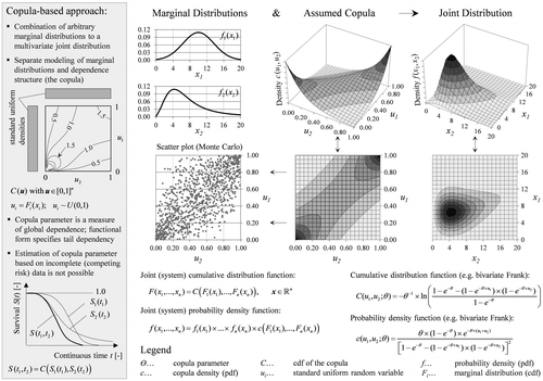
Figure 15. Combination of arbitrary marginal distributions to a multivariate joint distribution using copula (dependence) function.

Figure 16. Histrogram of the generated service life data (a), perspective (b) and contour plots (c) of the joint survival density based on a fitted Frank copula to the true data. Estimation of the marginal survival functions with the competing risk data and an assumed (fitted) copula using copula-graphic estimator (d).
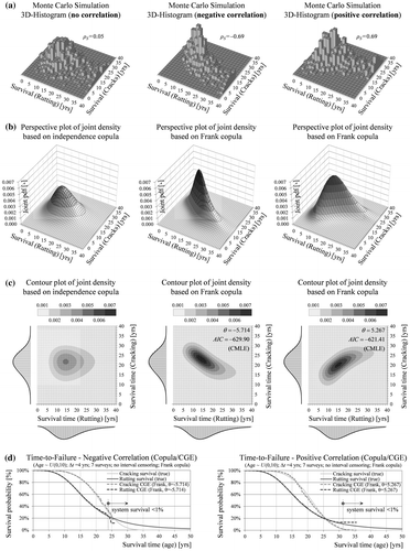
Figure 16. Histrogram of the generated service life data (a), perspective (b) and contour plots (c) of the joint survival density based on a fitted Frank copula to the true data. Estimation of the marginal survival functions with the competing risk data and an assumed (fitted) copula using copula-graphic estimator (d).
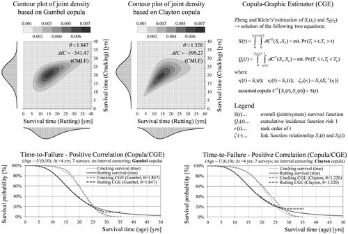
Figure 17. Definition of the copula-graphic estimator and sensitivity of the survival estimates to the functional form of the copula.

Figure 17. Definition of the copula-graphic estimator and sensitivity of the survival estimates to the functional form of the copula.