Figures & data
Figure 1. Overview of the developed performance, cost, duration and traffic models as modules of a holistic PMS, together with the sequence of computations from input to output.
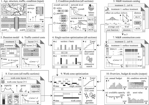
Figure 2. Overall service life (a) and dominant failure cause (b) resulting from the distress-specific service life distributions (c) and the correlations between these distributions (d).
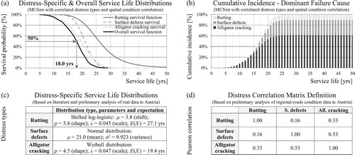
Figure 3. Positive serial correlation (а) vs. no serial correlation (b) of rutting service life for a 3-km road segment with partial autocorrelation function for the two cases (c). Fitting of autoregressive (2) process to real-world data with the estimated autoregressive parameters (d) and graphical representation of the road segment simultaneously exhibiting serial correlation and distress correlation (e).
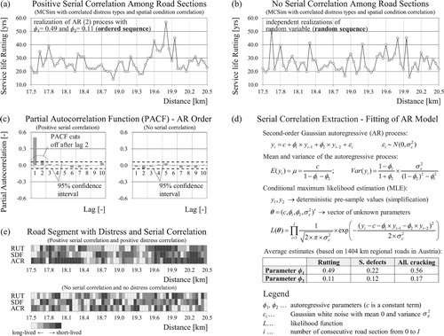
Figure 4. M&R treatment alternatives, characterised by depth of repair, effect (restore/delay) on the different distress types and technical applicability (decision tree).
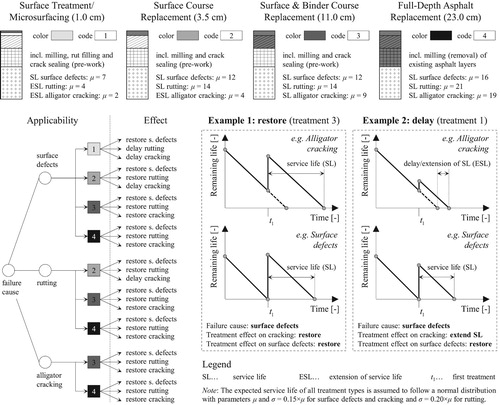
Figure 5. Bottom-up M&R construction cost calculation based on price lists and contractor’s bid prices from Austria. Unit costs (a) and total project costs (b) as a function of the project area for the considered four treatment types.
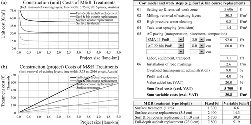
Figure 6. Common exterior-lane work-zone layouts on Austrian freeways (simplified) with corresponding speed limits, channelising devices and roadway capacity values (a,b). TTCCs derived by bottom-up approach as a function of the project length (c,d).
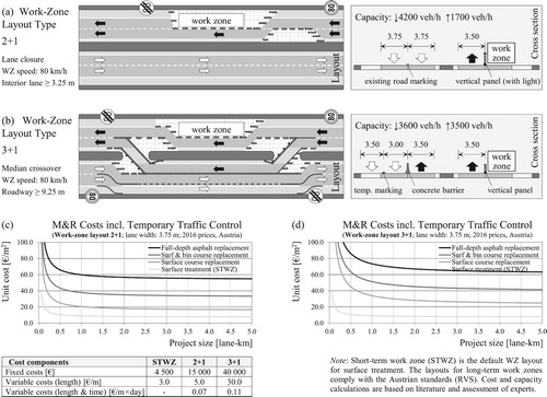
Figure 7. Derivation of the work-zone duration model (a,b) using production rates from the literature and accounting for days lost due to adverse weather conditions based on an extensive analysis of 180 weather stations over nine years in Austria (c).
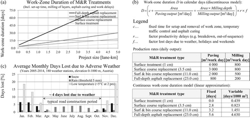
Figure 8. User costs incorporating TDC, VOC, EC and CC derived by bottom-up approach as a function of the project length for a single day (a,b) and for the total project duration by treatment type (c,d). Different traffic volumes and work-zone layouts lead to different parameters of the user-cost functions given in the table.
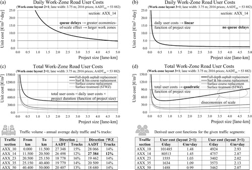
Figure 9. Methodology for M&R optimisation on a single road section for multiple distress types based on average costs, condition thresholds and treatment applicability considerations.
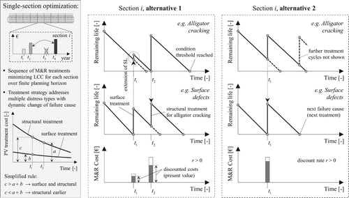
Figure 10. Methodology for optimisation of M&R treatment type, timing and work zones for multiple distress types based on economies-of-scale cost functions, condition thresholds and treatment applicability considerations.
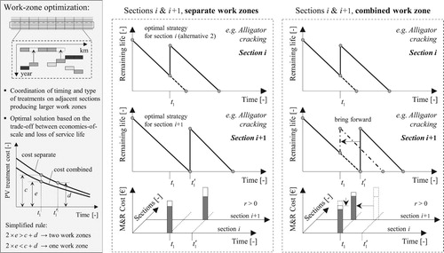
Figure 11. Size, characteristics and complexity of the formulated optimisation problem. Simple example with 10 sections and evaluation of the objective function for just one decision variable (timing for section 6) and for two decision variables (sections 5 and 6).
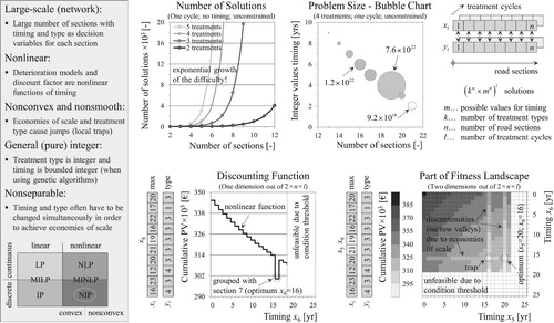
Figure 12. General overview of genetic algorithms: simplified example of steady-state GA, as well as most common operators for mutation, parent selection and crossover.
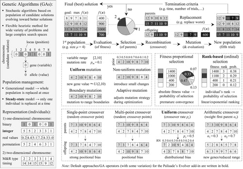
Figure 13. Results of the optimisation for a single road section (randomly chosen) with remaining life (a,c,e), expenditure stream (b,d) and present value (f) prior (basic) and after the optimization.
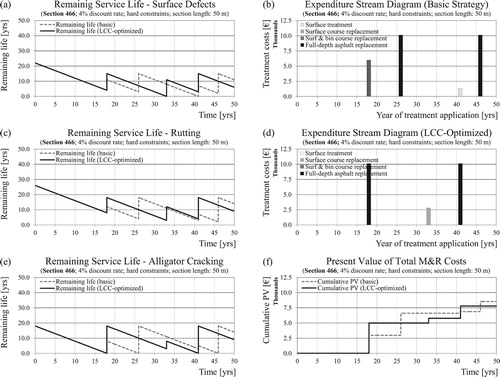
Figure 14. Results of the work-zone optimization for a segment of 60 road sections (randomly chosen) and 4% discount rate displaying only the first treatment of the life cycle for the cases of no optimization (a), minimum M&R costs (b), minimum total agency costs (c) and minimum total agency costs with soft constraints for alligator cracking (d).
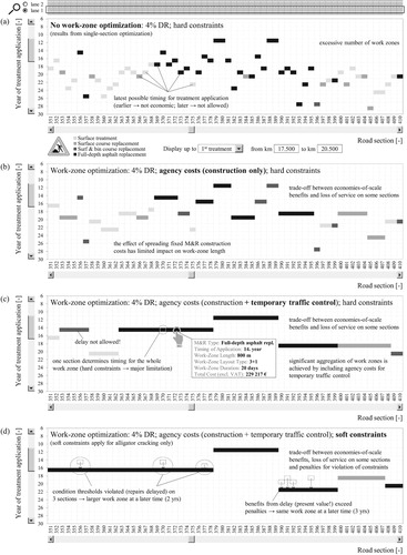
Figure 15. Distress-specific condition distributions for all sections in the cases of no-work zone optimization (a,c,e) and optimal work zones (b,d,f) using power functions to compute intermediate conditions.
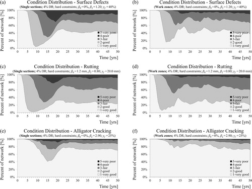
Figure 16. Effect of lower (a) and higher (b) than 4% discount rates on optimal work zones, treatment types and timings for the case of minimum total agency costs and hard constraints.
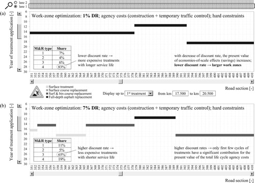
Figure 17. Number of work zones in different length classes by type of treatment for cases of different discount rates (a,b,c), soft constraints (d) and minimum M&R costs (e).
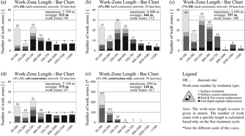
Figure 18. Effect of considering user costs together with agency costs in the work-zone optimization for layout 2 + 1 (a) and layout 3 + 1 (b) and a given traffic section (AXX_14). Selection of a work-zone layout based on total (agency plus user) costs.
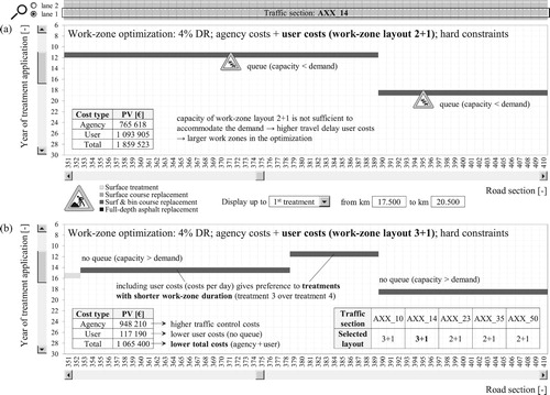
Figure 19. Comparison of work zones, annual budget and distribution of treatment types for the standard case of minimum total agency costs, hard constraints and 4% discount rate (a,b) and for the case of enhanced design life for alligator cracking under the same conditions (c,d) with display of the first three treatment cycles.
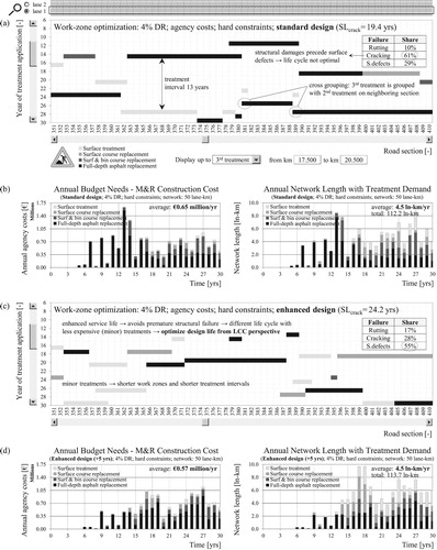
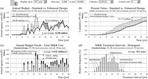
Figure 20. Potential savings as a result of avoiding premature structural failures by extending design life for alligator cracking in terms of annual budget (a) and present value (b). Total agency costs including TTCC (c) with histogram of treatment intervals (d) in the standard design case.