Tracking ∼200 years of water quality in Muskrat Lake, a eutrophic lake trout lake in Ontario (Canada) with cyanobacterial blooms

Figures & data

Figure 1. Map of region surrounding Muskrat Lake (Ontario, Canada), with shaded areas representing forested land. The arrow represents the direction of water flow, and the ⨂ marks the coring site at a depth of 33 m. Inset: Location of Muskrat Lake in Ontario (inverted black triangle) with Ottawa, Ontario, Canada, marked with a star.

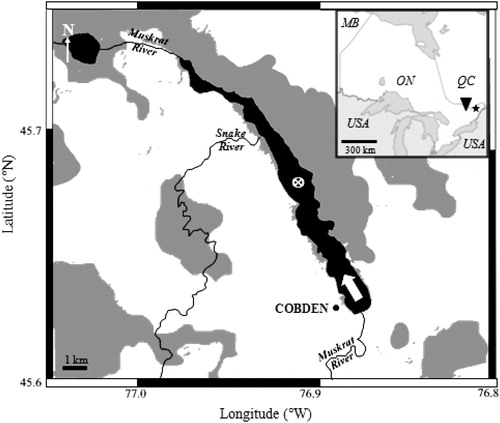
Figure 2. (a) Measured spring epilimnetic total phosphorus concentrations ([TP]_epi) averaged per decade, with the number of measurements noted at the bottom of each column. (b) Measured isopleths of 10 C water temperature (black solid line), 6 mg/L dissolved oxygen (black dashed line), <1 mg/L dissolved oxygen (gray striped area), and a dark gray shaded region of optimal late-summer lake trout optimal oxythermal habitat (temperature <10 C, dissolved oxygen >6 mg/L; Evans et al. 1991).

Figure 3. ²¹⁰Pb radiometric dating analysis of the Muskrat Lake sediment core, retrieved in July 2017. (a) Radioisotope activities by sediment depth and (b) estimated sediment age by depth as determined using the constant rate of supply (CRS) model for the Muskrat Lake sediment core (error bars indicating uncertainty in the date estimate).

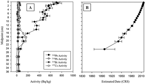
Figure 4. Mean annual air temperature (MAAT) from 1880 to 2017 in Killaloe, Ontario (gray points; ECCC 2019). The 1880–2017 average MAAT is indicated by the dotted horizontal gray line. The fitted values of the generalized additive model used to visualize the trend in MAAT (r²_adj = 0.59) is indicated with a solid line. The significant increasing trend is indicated by the thick black line.

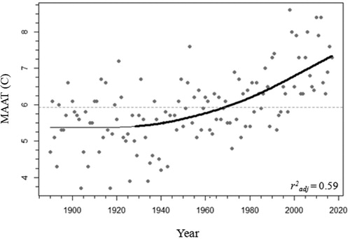
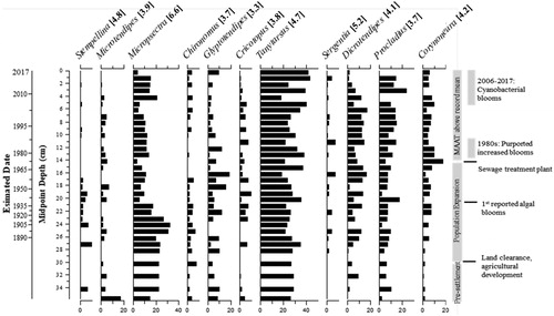
Figure 5. Simplified stratigraphy of diatom assemblages scaled by depth (with secondary axis of CRS-estimated ²¹⁰Pb dates) showing the relative abundances of the most common taxa. Taxa are ordered from high (lower left) to low (upper right) “optima,” approximated by canonical correspondence analysis (CCA) axis 1 species scores (CCA constrained to depth). Bold numbers in square brackets are estimated total phosphorus (TP) optima (µg/L) based on Reavie et al. (1995), Reavie et al. (2006), and Cumming et al. (2015). Numbers in parentheses depict the number of taxa in the grouping: Small cyclotelloid taxa (Lindavia ocellata, L. michiganiana, L. comensis, and Cyclotella cyclopuncta), benthic fragilarioid taxa (Staurosira construens, Staurosirella pinnata, and Pseudostaurosira brevistriata), and elongate planktonic Fragilaria taxa (F. capucina, F. ulna, and F. delicatissima) are grouped for display but are separate for statistical analyses. Horizontal lines depict CONISS zones with solid lines showing important zones identified by broken-stick analysis. The estimated timing of important historical events is given to the right of the diatom profile. Dates beyond ∼120 years were extrapolated but are not displayed; ca. 1850 is approximately 30 cm.

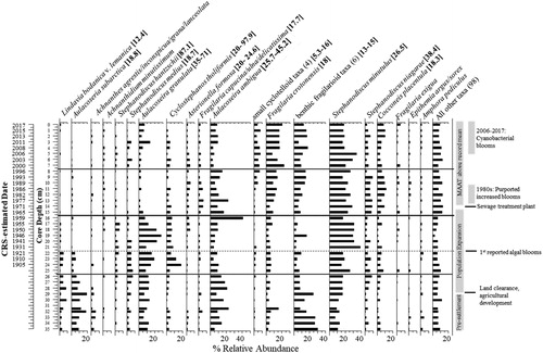
Figure 6. Species scores of principal component analysis (PCA) axes 1 and 2 for sedimentary (a, b) diatom and (c, d) chironomid assemblages, respectively. (e) The deviation in inferred values from the average pre-1850 (pre ∼30 cm) values for visual range spectroscopy (VRS)-inferred chlorophyll a trends. (f) Chironomid-inferred volume-weighted hypolimnetic oxygen (CI-VWHO) with the average for before ca. 1850 shown by a gray line, where black points represent good analogs, open points represent poor analogs, “X” markers indicate very poor analogs in the reconstruction, and error bars represent the 1.9 mg/L RSME of the Quinlan and Smol (2001b) model (see also Figure S2). (g) Deviation from the pre-1850 average CI-VWHO where black points represent good analogs, open points represent poor analogs, and “X” markers indicate very poor analogs in the reconstruction.

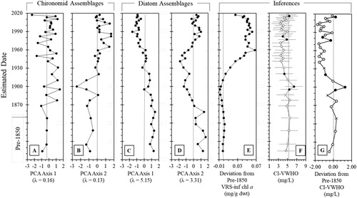
Figure 7. Simplified sedimentary chironomid (Diptera: Chironomidae) profile showing the relative abundances of the most common taxa ordered by weighted average from left to right. Bold numbers in square brackets are estimated end-of-summer volume-weighted hypolimnetic oxygen (VWHO) optima (mg/L) based on Quinlan and Smol (2001a). Taxa were grouped by genus for display but separated into the smallest taxonomic groups (e.g., species) for statistical analyses. The constrained incremental sum of squares (CONISS) is on the far right. Broken-stick analysis did not identify biostratigraphic zones (Bennett 1996). ²¹⁰Pb-estimated CRS dates and midpoint depths are on the y-axis. Dates beyond ∼120 years were extrapolated but are not displayed; ca. 1850 is approximately 30 cm.

Evans DO, Casselman JM, Wilcox CC. 1991. Effects of exploitation, loss of nursery habitat, and stocking on the dynamics and productivity of lake trout populations in Ontario lakes. Peterborough (ON): Ontario Ministry of Natural Resources; 103p.

 Google Scholar

Environment and Climate Change Canada (ECCC). 2019. Historical climate data: Killaloe, Ontario (station ID 6105976). Available from https://climate-change.canada.ca/climate-data/#/adjusted-station-data.

 Google Scholar

Reavie ED, Hall RI, Smol JP. 1995. An expanded weighted-averaging model for inferring past total phosphorus concentrations from diatom assemblages in eutrophic British Columbia (Canada) lakes. J Paleolimnol. 14(1):49–67. doi:10.1007/BF00682593.

 Web of Science ®Google Scholar

Reavie ED, Neill KE, Little JL, Smol JP. 2006. Cultural eutrophication trends in three southeastern Ontario lakes: a paleolimnological perspective. Lake Reserv Manage. 22(1):44–58. doi:10.1080/07438140609353883.

 Web of Science ®Google Scholar

Cumming BF, Laird KR, Gregory-Eaves I, Simpson KG, Sokal MA, Nordin RN, Walker IR. 2015. Tracking past changes in lake-water phosphorus with a 251-lake calibration dataset in British Columbia: tool development and application in a multiproxy assessment of eutrophication and recovery in Osoyoos Lake, a transboundary lake in Western North America. Front Ecol Evol. 3:84.

 Web of Science ®Google Scholar

Quinlan R, Smol JP. 2001b. Setting minimum head capsule abundance and taxa deletion criteria in chironomid-based inference models. J Paleolimnol. 26(3):327–342.

 Web of Science ®Google Scholar

Quinlan R, Smol JP. 2001a. Chironomid-based inference models for estimating end-of-summer hypolimnetic oxygen from south-central Ontario Shield lakes. Freshwater Biol. 46(11):1529–1551. doi:10.1046/j.1365-2427.2001.00763.x.

 Web of Science ®Google Scholar

Bennett KD. 1996. Determination of the number of zones in a biostratigraphical sequence. New Phytol. 132(1):155–170. doi:10.1111/j.1469-8137.1996.tb04521.x.

 PubMed Web of Science ®Google Scholar